Curiousily

Building a Cat Detector using Convolutional Neural Networks | TensorFlow for Hackers - Part III

24.04.2017 — Deep Learning, Neural Networks, TensorFlow, Python — 3 min read

Have you ever stood still, contemplating about how cool would it be to build a model that can distinguish cats from dogs? Don’t be shy now! Of course you did! Let’s get going!

Cat or a dog?

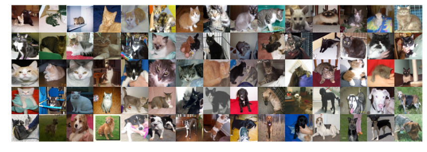
We have 25,000 labeled pictures of dogs and cats. The data comes from Kaggle’s Dogs vs Cats challenge. That’s how a bunch of them look like:

source: subsubroutine.com

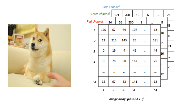
Let’s focus on a specific image. Each picture can be represented as a 3-dimensional array. We will resize all training image to 50 x 50 pixels. Here’s a crazy example:

source: subsubroutine.com

Additionally, we will remove all color and turn them pictures into grayscale ones. First things first, let’s prepare our environment:

Setting up

Download the train and test zip files from Kaggle and extract them into your current working directory.

1import cv2
2import numpy as np
3import os
4from random import shuffle
5from tqdm import tqdm
6import tensorflow as tf
7import matplotlib.pyplot as plt
8
9import tflearn
10from tflearn.layers.conv import conv_2d, max_pool_2d
11from tflearn.layers.core import input_data, dropout, fully_connected
12from tflearn.layers.estimator import regression
13
14%matplotlib inline
15
16TRAIN_DIR = 'train'
17TEST_DIR = 'test'
18IMG_SIZE = 50
19LR = 1e-3
20
21MODEL_NAME = 'dogs-vs-cats-convnet'
22tf.__version__

1'1.1.0'

Image preprocessing

We have 25,000 images for training and 12,500 for testing. Let’s create a function that encodes the labels of the training images:

1def create_label(image_name):
2    """ Create an one-hot encoded vector from image name """
3    word_label = image_name.split('.')[-3]
4    if word_label == 'cat':
5        return np.array([1,0])
6    elif word_label == 'dog':
7        return np.array([0,1])

Now, for the actual reading of training and test data. Every image will be resized to 50 x 50 pixels and read as grayscale:

1def create_train_data():
2    training_data = []
3    for img in tqdm(os.listdir(TRAIN_DIR)):
4        path = os.path.join(TRAIN_DIR, img)
5        img_data = cv2.imread(path, cv2.IMREAD_GRAYSCALE)
6        img_data = cv2.resize(img_data, (IMG_SIZE, IMG_SIZE))
7        training_data.append([np.array(img_data), create_label(img)])
8    shuffle(training_data)
9    np.save('train_data.npy', training_data)
10    return training_data

1def create_test_data():
2    testing_data = []
3    for img in tqdm(os.listdir(TEST_DIR)):
4        path = os.path.join(TEST_DIR,img)
5        img_num = img.split('.')[0]
6        img_data = cv2.imread(path, cv2.IMREAD_GRAYSCALE)
7        img_data = cv2.resize(img_data, (IMG_SIZE, IMG_SIZE))
8        testing_data.append([np.array(img_data), img_num])
9
10    shuffle(testing_data)
11    np.save('test_data.npy', testing_data)
12    return testing_data

Now, let’s split the data. 24,500 images for training and 500 for testing. We also need to reshape the data appropriately for TensorFlow:

1# If dataset is not created:
2train_data = create_train_data()
3test_data = create_test_data()
4
5# If you have already created the dataset:
6# train_data = np.load('train_data.npy')
7# test_data = np.load('test_data.npy')
8
9train = train_data[:-500]
10test = train_data[-500:]
11
12X_train = np.array([i[0] for i in train]).reshape(-1, IMG_SIZE, IMG_SIZE, 1)
13y_train = [i[1] for i in train]
14
15X_test = np.array([i[0] for i in test]).reshape(-1, IMG_SIZE, IMG_SIZE, 1)
16y_test = [i[1] for i in test]

1100%|██████████| 25000/25000 [01:04<00:00, 386.67it/s]
2100%|██████████| 12500/12500 [00:32<00:00, 387.32it/s]

Convolutional Neural Nets

How will we do it? Isn’t that just too hard of a task? Convolutional Neural Networks to the rescue!

In the past, people had to think of and code different kinds of features that might be relevant to the task at hand. Examples of that would be whiskers, ears, tails, legs, fur type detectors. These days, we can just use Convolutional NNs. They can learn features from raw data. How do they work?

Ok, got it? It was a great explanation. You can think of convolutions as small sliding lenses (let’s say a 5 x 5) that are “activated” when are placed above some feature that is familiar to them. That way, convolutions can make sense of larger portions of the image, not just single pixels.

Building our model

Finally, the fun part begins! We will use tflearn to build our Convolutional Neural Network. One additional bonus will be the use of a Dropout layer. Here’s the model:

1tf.reset_default_graph()
2
3convnet = input_data(shape=[None, IMG_SIZE, IMG_SIZE, 1], name='input')
4
5convnet = conv_2d(convnet, 32, 5, activation='relu')
6convnet = max_pool_2d(convnet, 5)
7
8convnet = conv_2d(convnet, 64, 5, activation='relu')
9convnet = max_pool_2d(convnet, 5)
10
11convnet = fully_connected(convnet, 1024, activation='relu')
12convnet = dropout(convnet, 0.8)
13
14convnet = fully_connected(convnet, 2, activation='softmax')
15convnet = regression(convnet, optimizer='adam', learning_rate=LR, loss='categorical_crossentropy', name='targets')
16
17model = tflearn.DNN(convnet, tensorboard_dir='log', tensorboard_verbose=0)
18
19model.fit({'input': X_train}, {'targets': y_train}, n_epoch=10,
20          validation_set=({'input': X_test}, {'targets': y_test}),
21          snapshot_step=500, show_metric=True, run_id=MODEL_NAME)

1Training Step: 3829  | total loss: [1m[32m11.45499[0m[0m | time: 35.818s
2| Adam | epoch: 010 | loss: 11.45499 - acc: 0.5025 -- iter: 24448/24500
3Training Step: 3830  | total loss: [1m[32m11.49676[0m[0m | time: 36.938s
4| Adam | epoch: 010 | loss: 11.49676 - acc: 0.5007 | val_loss: 11.60503 - val_acc: 0.4960 -- iter: 24500/24500
5--

We resized our images to 50 x 50 x 1 matrices and that is the size of the input we are using.

Next, a convolutional layer with 32 filters and stride = 5 is created. The activation function is ReLU. Right after that, a max pool layer is added. That same trickery is repeated again with 64 filters.

Next, a fully-connected layer with 1024 neurons is added. Finally, a dropout layer with keep probability of 0.8 is used to finish our model.

We use Adam as optimizer with learning rate set to 0.001. Our loss function is categorical cross entropy. Finally, we train our Deep Neural Net for 10 epochs.

All that is great, but our validation accuracy doesn’t seem that good. Flipping a coin might be a better model than the one we created. Let’s go bigger and better (hopefully):

Building our (bigger) model

1tf.reset_default_graph()
2
3convnet = input_data(shape=[None, IMG_SIZE, IMG_SIZE, 1], name='input')
4
5convnet = conv_2d(convnet, 32, 5, activation='relu')
6convnet = max_pool_2d(convnet, 5)
7
8convnet = conv_2d(convnet, 64, 5, activation='relu')
9convnet = max_pool_2d(convnet, 5)
10
11convnet = conv_2d(convnet, 128, 5, activation='relu')
12convnet = max_pool_2d(convnet, 5)
13
14convnet = conv_2d(convnet, 64, 5, activation='relu')
15convnet = max_pool_2d(convnet, 5)
16
17convnet = conv_2d(convnet, 32, 5, activation='relu')
18convnet = max_pool_2d(convnet, 5)
19
20convnet = fully_connected(convnet, 1024, activation='relu')
21convnet = dropout(convnet, 0.8)
22
23convnet = fully_connected(convnet, 2, activation='softmax')
24convnet = regression(convnet, optimizer='adam', learning_rate=LR, loss='categorical_crossentropy', name='targets')
25
26model = tflearn.DNN(convnet, tensorboard_dir='log', tensorboard_verbose=0)
27
28model.fit({'input': X_train}, {'targets': y_train}, n_epoch=10,
29          validation_set=({'input': X_test}, {'targets': y_test}),
30          snapshot_step=500, show_metric=True, run_id=MODEL_NAME)

1Training Step: 3829  | total loss: [1m[32m0.34434[0m[0m | time: 44.501s
2| Adam | epoch: 010 | loss: 0.34434 - acc: 0.8466 -- iter: 24448/24500
3Training Step: 3830  | total loss: [1m[32m0.35046[0m[0m | time: 45.619s
4| Adam | epoch: 010 | loss: 0.35046 - acc: 0.8432 | val_loss: 0.50006 - val_acc: 0.7860 -- iter: 24500/24500
5--

That is pretty much the same model. One difference is the number of convolutional and max pool layers we added. So, our model has much more parameters and can learn more complex functions. One proof of that is the validation accuracy that is around 0.8. Let’s take our model for a spin!

Did we do well?

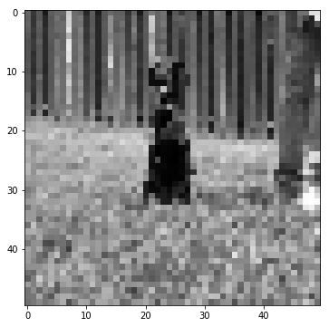
Let’s have a look at a single prediction:

1d = test_data[0]
2img_data, img_num = d
3
4data = img_data.reshape(IMG_SIZE, IMG_SIZE, 1)
5prediction = model.predict([data])[0]
6
7fig = plt.figure(figsize=(6, 6))
8ax = fig.add_subplot(111)
9ax.imshow(img_data, cmap="gray")
10print(f"cat: {prediction[0]}, dog: {prediction[1]}")

1cat: 0.8773844838142395, dog: 0.12261549383401871

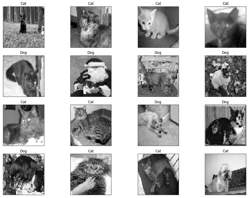
That doesn’t look right. How about some more predictions:

1fig=plt.figure(figsize=(16, 12))
2
3for num, data in enumerate(test_data[:16]):
4
5    img_num = data[1]
6    img_data = data[0]
7
8    y = fig.add_subplot(4, 4, num+1)
9    orig = img_data
10    data = img_data.reshape(IMG_SIZE, IMG_SIZE, 1)
11    model_out = model.predict([data])[0]
12
13    if np.argmax(model_out) == 1:
14        str_label='Dog'
15    else:
16        str_label='Cat'
17
18    y.imshow(orig, cmap='gray')
19    plt.title(str_label)
20    y.axes.get_xaxis().set_visible(False)
21    y.axes.get_yaxis().set_visible(False)
22plt.show()

Conclusion

There you have it! Santa is a dog! More importantly, you built a model that can distinguish cats from dogs using only raw pixels (albeit, with a tiny bit of preprocessing). Additionally, it trains pretty fast on relatively old machines! Can you improve the model? Maybe change the architecture, keep probability parameter of the Dropout layer or the optimizer? What results did you get?

The only thing left for you to do is snap a photo of your cat or dog and run it through your model. Was the net correct?

References

An Intuitive Explanation of Convolutional Neural Networks
CS231n - Convolutional Neural Networks (CNNs / ConvNets)
Cats and dogs and convolutional neural networks
Gradient-based learning applied to document recognition

Want to be a Machine Learning expert?

Join the weekly newsletter on Data Science, Deep Learning and Machine Learning in your inbox, curated by me! Chosen by 10,000+ Machine Learning practitioners. (There might be some exclusive content, too!)

You'll never get spam from me

Hacker's Guide to Neural Networks in JavaScript

Build Machine Learning models (especially Deep Neural Networks) that you can easily integrate with existing or new web apps. Think of your ReactJs, Vue, or Angular app enhanced with the power of Machine Learning models.

Get SH*T Done with PyTorch

Learn how to solve real-world problems with Deep Learning models (NLP, Computer Vision, and Time Series). Go from prototyping to deployment with PyTorch and Python!

Hacker's Guide to Machine Learning with Python

This book brings the fundamentals of Machine Learning to you, using tools and techniques used to solve real-world problems in Computer Vision, Natural Language Processing, and Time Series analysis. The skills taught in this book will lay the foundation for you to advance your journey to Machine Learning Mastery!

Hands-On Machine Learning from Scratch

This book will guide you on your journey to deeper Machine Learning understanding by developing algorithms in Python from scratch! Learn why and when Machine learning is the right tool for the job and how to improve low performing models!