TL;DR Build a Logistic Regression model in TensorFlow.js using the high-level layers API, and predict whether or not a patient has Diabetes. Learn how to visualize the data, create a Dataset, train and evaluate multiple models.

You’ve been living in this forgotten city for the past 8+ months. You never felt comfortable anywhere but home. However, this place sets a new standard. The constant changes between dry and humid heat are killing you, fast.

The Internet connection is spotty at best, and you haven’t heard from your closed ones for more than two weeks. You have no idea how your partner is and how your kids are doing. You sometimes question the love for your country.

This morning you feel even worse. Constantly hungry and thirsty. You urinated four times, already, and your vision is somewhat blurry. It is not just today you were feeling like that for a week, at least.

You went to the doctor, and she said you might be having Diabetes. Both your mother and father suffer from it, so it seems likely to you. She wasn’t that sure and did a glucose test. Unfortunately, you’re being called and should go before the results are in.

You’re going away for two weeks. Only a couple of guys and your laptop! You have a couple of minutes and download a Diabetes patient dataset. You have TensorFlow.js already installed and a copy of the whole API. Can you build a model to predict whether or not you have Diabetes?

Run the complete source code for this tutorial right in your browser:

Diabetes data

Diabetes mellitus (DM), commonly known as diabetes, is a group of metabolic disorders characterized by high blood sugar levels over a prolonged period. Symptoms of high blood sugar include frequent urination, increased thirst, and increased hunger. If left untreated, diabetes can cause many complications. Acute complications can include diabetic ketoacidosis, hyperosmolar hyperglycemic state, or death. Serious long-term complications include cardiovascular disease, stroke, chronic kidney disease, foot ulcers, and damage to the eyes.

As of 2017, an estimated 425 million people had diabetes worldwide (around 5.5%)

Our data comes from Kaggle but was first introduced in the paper: Using the ADAP Learning Algorithm to Forecast the Onset of Diabetes Mellitus

The population for this study was the Pima Indian population near Phoenix, Arizona. That population has been under continuous study since 1965 by the National Institute of Diabetes and Digestive and Kidney Diseases because of its high incidence rate of diabetes. Each community resident over 5 years of age was asked to undergo a standardized examination every two years, which included an oral glucose tolerance test. Diabetes was diagnosed according to World Health Organization Criteria; that is, if the 2 hour post-load plasma glucose was at least 200 mg/dl (11.1 mmol/l) at any survey examination or if the Indian Health Service Hospital serving the community found a glucose concentration of at least 200 mg/dl during the course of routine medical care.

Here is a summary of the data:

• Pregnancies - Number of times pregnant
• Glucose - Plasma glucose concentration a 2 hours in an oral glucose tolerance test
• BloodPressure - Diastolic blood pressure (mm Hg)
• SkinThickness - Triceps skin fold thickness (mm)
• Insulin - 2-Hour serum insulin (mu U/ml)
• BMI - Body mass index ($\frac{weight}{height^2}$ in kg/m)
• DiabetesPedigreeFunction - Diabetes Pedigree Function (DPF)
• Age - Age (years)
• Outcome - Class variable (0 - healthy or 1 - diabetic)

According to Estimating Probabilities of Diabetes Mellitus Using Neural Networks paper, the DPF provides:

A synthesis of the diabetes mellitus history in relatives and the genetic relationship of those relatives to the subject. The DPF uses information from parents, grandparents, siblings, aunts and uncles, and first cousins. It provides a measure of the expected genetic influence of affected and unaffected relatives on the subject’s eventual diabetes risk.

Who are Pima Indians?

The Pima (or Akimel Oʼodham, also spelled Akimel Oʼotham, “River People”, formerly known as Pima) are a group of Native Americans living in an area consisting of what is now central and southern Arizona. The majority population of the surviving two bands of the Akimel Oʼodham are based in two reservations: the Keli Akimel Oʼotham on the Gila River Indian Community (GRIC) and the On’k Akimel Oʼodham on the Salt River Pima-Maricopa Indian Community (SRPMIC).

Read the data

We’ll use the Papa Parse library to read the csv file. Unfortunately, Papa Parse doesn’t work well with await/async. Let’s change that:

1import * as Papa from "papaparse"
2
3Papa.parsePromise = function (file) {
4  return new Promise(function (complete, error) {
5    Papa.parse(file, {
6      header: true,
7      download: true,
8      dynamicTyping: true,
9      complete,
10      error,
11    })
12  })
13}

We use the dynamicTyping parameter to instruct Papa Parse to convert the numbers in the dataset from strings. Let’s define a function that loads the data:

1const loadData = async () => {
2  const csv = await Papa.parsePromise(
3    "https://raw.githubusercontent.com/curiousily/Logistic-Regression-with-TensorFlow-js/master/src/data/diabetes.csv"
4  )
5  return csv.data
6}

and use it:

1const data = await loadData()

Good job! We have the data, let get familiar with it!

Exploration

While tfjs-vis is nice and well integrated with TensorFlow.js, it lacks (at the time of this writing) a ton of features you might need - overlay plots, color changes, scale customization, etc. That’s why we’ll use Plotly’s Javascript library to make some beautiful plots for our data exploration.

Let’s have a look at the distribution of healthy vs diabetic people:

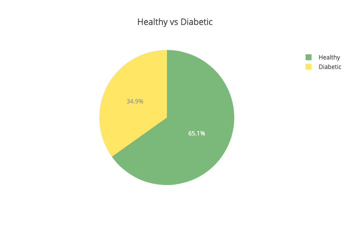
Little above 65% of the patients in our dataset are healthy. That means that our model should be more accurate than 65% of the time, to be any good. Next up - the insulin levels:

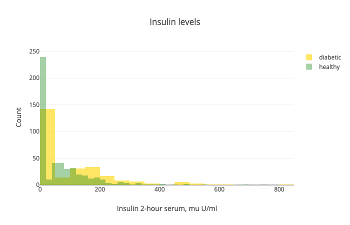
Note that there is a big overlap between the two distributions. Also, we have a lot of 0s in the dataset. Seems like we have a lot of missing values. NaNs are replaced with 0s.

Another important one is the glucose levels after the test:

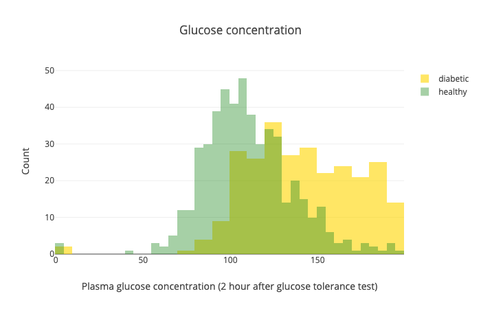
While there is some overlap, this test seems like it separates the healthy from diabetic patients pretty well.

Let’s have a look at the age:

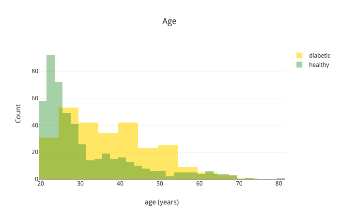
Generally speaking, it seems like older people are more likely to have diabetes.

Maybe we should take a look at the relationship between age and glucose levels:

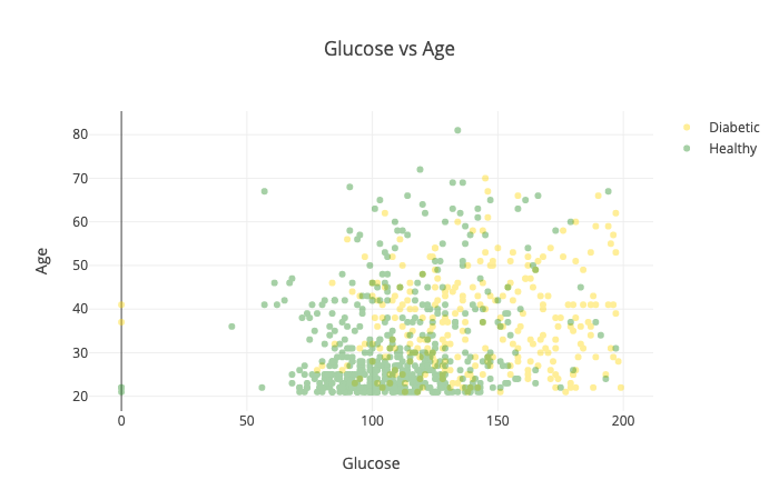
The combination of those two seems to separate healthy and diabetic patients very well. That might do wonders for our model.

Another combination you might want to try is the skin thickness vs BMI:

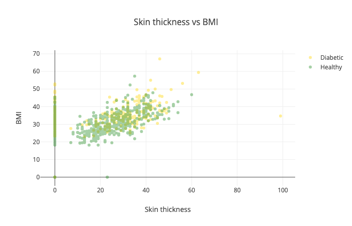
Yep, this one is horrible and doesn’t tell us much :)

Preprocessing

Currently, our data sits in an array of objects. Unfortunately, TensorFlow doesn’t work well with those. Luckily, there is the tfjs-data package. We’re going to create a Dataset from our CSV file and use it to train our model with the createDatasets() function:

1const createDataSets = (data, features, testSize, batchSize) => {
2  ...
3};

The features parameter specifies which columns are in the dataset. testSize is the fraction of the data that is going to be used for testing. batchSize controls the number of data points when the dataset is split into chunks (batches).

Let’s start by extracting the features from the data:

1const X = data.map(r =>
2  features.map(f => {
3    const val = r[f]
4    return val === undefined ? 0 : val
5  })
6)

We’re replacing missing values in our features with 0s. You might try to train your model without this step and see what happens?

Let’s prepare the labels:

1const y = data.map(r => {
2  const outcome = r.Outcome === undefined ? 0 : r.Outcome
3  return oneHot(outcome)
4})

Here’s the definition of oneHot:

1const oneHot = outcome => Array.from(tf.oneHot(outcome, 2).dataSync())

One-hot encoding turns categorical variables (healthy - 0 and diabetic - 1) into an array where 1 corresponds to the position of the category and all other variables are 0. Here are some examples:

11 // diabetic =>
2;[0, 1]

10 // healthy =>
2;[1, 0]

Let’s create a Dataset from our data:

1const ds = tf.data
2  .zip({ xs: tf.data.array(X), ys: tf.data.array(y) })
3  .shuffle(data.length, 42)

Note that we also shuffle the data with a seed of 42 :)

Finally, let’s split the data into training and validation datasets:

1const splitIdx = parseInt((1 - testSize) * data.length, 10)
2
3return [
4  ds.take(splitIdx).batch(batchSize),
5  ds.skip(splitIdx + 1).batch(batchSize),
6  tf.tensor(X.slice(splitIdx)),
7  tf.tensor(y.slice(splitIdx)),
8]

We use take to create the training dataset, skip to omit the training examples for the validation dataset and finally, split the data into chunks using batch.

Additionally, we return data for testing our model (more on this later).

Logistic Regression

Logistic Regression (contrary to its name) allows you to get binary (yes/no) answers from your data. Moreover, it gives you the probability for each answer. Questions like:

• Is this email spam?
• Should I ask my boss for a higher salary?
• Does this patient have diabetes?
• Is this person a real friend?
• Does my partner cheat on me?
• Do I cheat on my partner?
• Do you get where I am getting at?

are answerable using Logistic Regression if sufficient data is available and you’re lucky enough to believe there are answers to all of these?

But I digress, let’s have a look at the mathematical formulation of the Logistic Regression. First, let’s start with the Linear Model:

where $x$ is the data we’re going to use to train our model, $b_1$ controls the slope and $b_0$ the interception point with the $y$ axis.

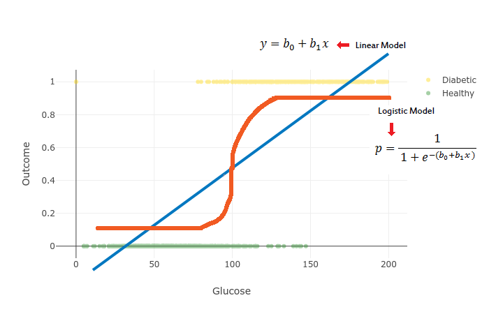
We’re going to use the softmax function to get probabilities out of the Linear Model and obtain a generalized model of Logistic Regression. Softmax Regression allows us to create a model with more than 2 output classes (binary response):

where $b_1$ defines the steepness of the curve and $b_0$ moves the curve left and right.

We want to use our data $X$ and some training magic to learn the parameters $b_1$ and $b_0$. Let’s use TensorFlow.js for that!

Note that this model will give us a probabilistic answer instead of just a binary response. You might decide to ignore a prediction if the model is not sure about it - e.g. below 80%.

Predicting diabetes

Let’s put the theory into practice by building a model into TensorFlow.js and predict the outcome for a patient.

The model

Remember that the key to building a Logistic Regression model was the Linear Model and applying a softmax function to it:

1const model = tf.sequential()
2model.add(
3  tf.layers.dense({
4    units: 2,
5    activation: "softmax",
6    inputShape: [featureCount],
7  })
8)

Note that we have 2 outputs because of the one-hot encoding and dynamic input count, based on the features we’ve chosen to train the model. Yes, it is that easy to build a Logistic Regression model in TensorFlow.js.

The next step is to compile the model:

1const optimizer = tf.train.adam(0.001)
2model.compile({
3  optimizer: optimizer,
4  loss: "binaryCrossentropy",
5  metrics: ["accuracy"],
6})

The training process of our model consists of minimizing the loss function. This gets done by the Adam optimizer we’re providing. Note that we’re providing a learning rate of 0.001.

The learning rate is known as a hyperparameter since it is a parameter you provide for your model to use. It controls how much each new update should “override” what your model already knows. Choosing the “correct” learning rate is somewhat of voodoo magic.

We’re using Cross-Entropy loss (known as log loss) to evaluate how well our model is doing. It (harshly) penalizes wrong answers given from classification models, based on the probabilities they give for each class. Here is the definition:

where $C$ is the number of classes, $y$ is a binary indicator if the class label is the correct classification for the observation and $p$ is the predicted probability that $o$ is of class $c$.

Note that we request from TensorFlow to record the accuracy metrics.

Training

Let’s use fitDataset to train our model using the training and validation datasets we’ve prepared:

1const trainLogs = []
2const lossContainer = document.getElementById("loss-cont")
3const accContainer = document.getElementById("acc-cont")
4
5await model.fitDataset(trainDs, {
6  epochs: 100,
7  validationData: validDs,
8  callbacks: {
9    onEpochEnd: async (epoch, logs) => {
10      trainLogs.push(logs)
11      tfvis.show.history(lossContainer, trainLogs, ["loss", "val_loss"])
12      tfvis.show.history(accContainer, trainLogs, ["acc", "val_acc"])
13    },
14  },
15})

We train our model for 100 epochs (number of times the whole training set is shown to the model) and record the training logs for visualization using the onEpochEnd callback.

We’re going to wrap all of this into a function called trainLogisticRegression which is defined as:

1const trainLogisticRegression = async (
2  featureCount,
3  trainDs,
4  validDs
5) => {
6...
7}

Evaluation

Let’s use everything we’ve built so far to evaluate how well our model is doing:

1const features = ["Glucose"]
2
3const [trainDs, validDs, xTest, yTest] = createDataSets(data, features, 0.1, 16)
4
5trainLogisticRegression(features.length, trainDs, validDs)

Note that we only use the glucose levels for training our model. Here are the results:

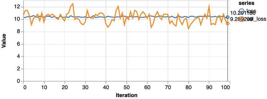
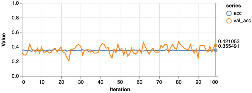
Not good at all. Our model performs worse than a dummy that predicts healthy 65% of the time. Also, the loss never really starts dropping. Let’s try with more data:

1const features = ["Glucose", "Age", "Insulin", "BloodPressure"]
2
3const [trainDs, validDs, xTest, yTest] = createDataSets(data, features, 0.1, 16)
4
5const model = await trainLogisticRegression(features.length, trainDs, validDs)

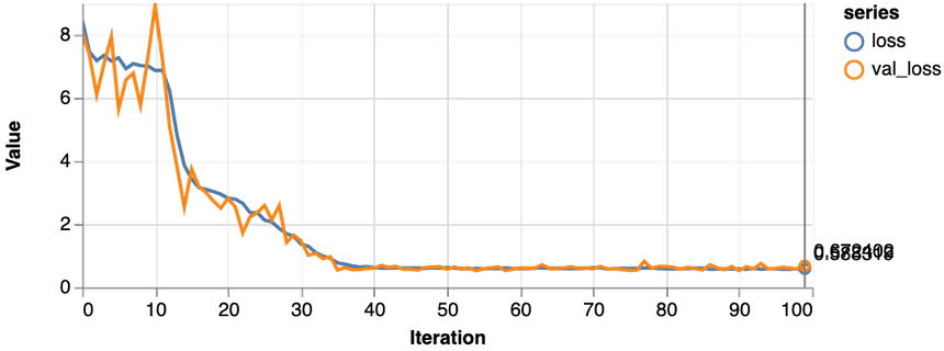
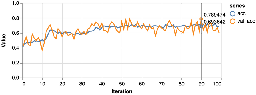
Much better, the loss value is reduced significantly during training, and we obtain about 79% accuracy on the validation set. Let’s take a closer look at the classification performance with a confusion matrix:

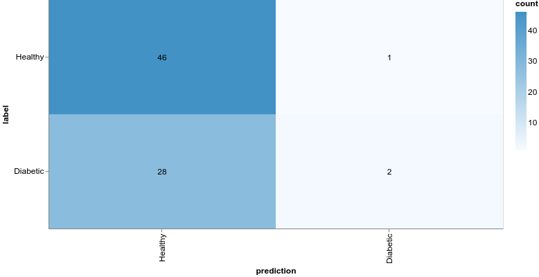
The confusion matrix can be obtained using the model predictions and test set:

1const preds = model.predict(xTest).argMax(-1)
2const labels = yTest.argMax(-1)
3
4const confusionMatrix = await tfvis.metrics.confusionMatrix(labels, preds)
5
6const container = document.getElementById("confusion-matrix")
7
8tfvis.render.confusionMatrix(container, {
9  values: confusionMatrix,
10  tickLabels: ["Healthy", "Diabetic"],
11})

Even though our model might’ve obtained better accuracy, the results are still horrible. Being healthy is vastly overpredicted compared to having diabetes. What if we try with a more complex model:

1const model = tf.sequential()
2
3model.add(
4  tf.layers.dense({
5    units: 12,
6    activation: "relu",
7    inputShape: [featureCount],
8  })
9)
10
11model.add(
12  tf.layers.dense({
13    units: 2,
14    activation: "softmax",
15  })
16)

Here is the confusion matrix for this model:

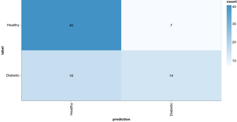
We’ll not look into this model for now, but note that we obtain much better results by increasing the complexity of the model.

Conclusion

Congratulations! You built and trained not one, but a couple of models, including Logistic Regression, that predicts whether or not a patient has Diabetes. You’ve also met the real-world - processing data, training and building models, are hard things to do. Moreover, not everything is predictable, no matter how many data points you have.

Run the complete source code for this tutorial right in your browser:

That said, there are ways to improve the process of building and training models. We know that using some techniques is better than others, in a certain context. Well, Machine Learning is nuanced :)

References

• Logistic Regression by Dr. Saed Sayad
• A Gentle Introduction to TensorFlow.js