TL;DR Learn how to do feature scaling, handle categorical data and do feature engineering with Pandas and Scikit-learn in Python. Use your skills to preprocess a housing dataset and build a model to predict prices.

I know, data preprocessing might not sound cool. You might just want to train Deep Neural Networks (or your favorite models). I am here to shatter your dreams, you’ll most likely spend a lot more time on data preprocessing and exploration than any other step of your Machine Learning workflow.

Since this step is so early in the process, screwing up here will lead to useless models. Garbage data in, garbage predictions out. A requirement for reaching your model’s full potential is proper cleaning, wrangling and analysis of the data.

This guide will introduce you to the most common and useful methods to preprocess your data. We’re going to look at three general techniques:

• Feature Scaling
• Handling Categorical Data
• Feature Engineering

Finally, we’re going to apply what we’ve learned on a real dataset and try to predict Melbourne housing prices. We’re going to compare the performance of a model with and without data preprocessing. How improtant data preparation really is?

Run the complete notebook in your browser

The complete project on GitHub

Feature Scaling

Feature scaling refers to the process of changing the range (normalization) of numerical features. There are different methods to do feature scaling. But first, why do you need to do it?

When Machine Learning algorithms measure distances between data points, the results may be dominated by the magnitude (scale) of the features instead of their values. Scaling the features to a similar range can fix the problem. Gradient Descent can converge faster when feature scaling is applied.

Use feature scaling when your algorithm calculates distances or is trained with Gradient Descent

How can we do feature scaling? Scikit-learn offers a couple of methods. We’ll use the following synthetic data to compare them:

1data = pd.DataFrame({
2    'Normal': np.random.normal(100, 50, 1000),
3    'Exponential': np.random.exponential(25, 1000),
4    'Uniform': np.random.uniform(-150, -50, 1000)
5})

Min-Max Normalization

One of the simplest and most widely used approaches is to scale each feature in the [0, 1] range. The scaled value is given by:

MinMaxScaler allows you to select the rescale range with the feature_range parameter:

1from sklearn.preprocessing import MinMaxScaler
2
3min_max_scaled = MinMaxScaler(feature_range=(0, 1)).fit_transform(data)

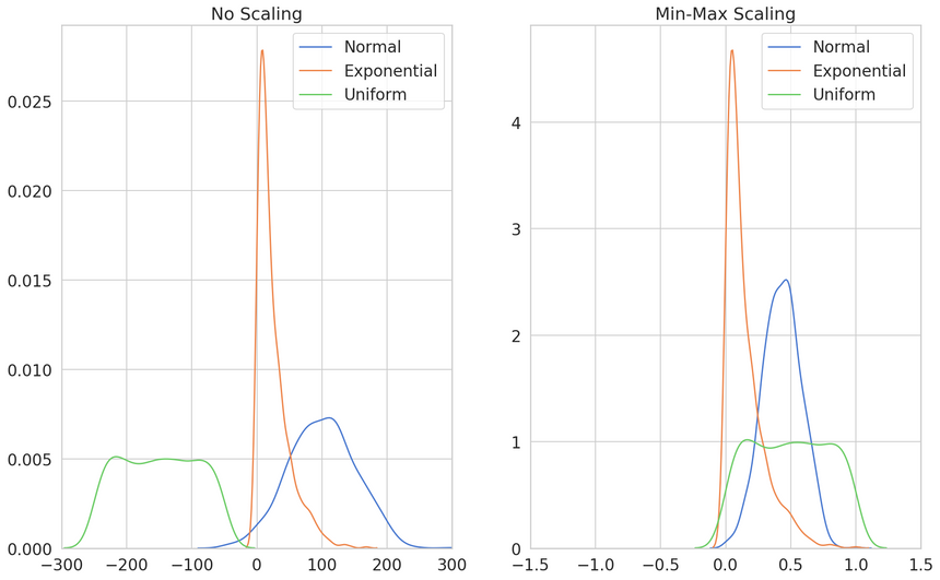
The scaled distributions do not overlap as much and their shape remains the same (except for the Normal).

This method preserves the shape of the original distribution and is sensitive to outliers.

Standardization

This method rescales a feature removing the mean and divides by standard deviation. It produces a distribution centered at 0 with a standard deviation of 1. Some Machine Learning algorithms (SVMs) assume features are in this range.

It is defined by:

You can use the StandarScaler like this:

1from sklearn.preprocessing import StandardScaler
2
3stand_scaled = StandardScaler().fit_transform(data)

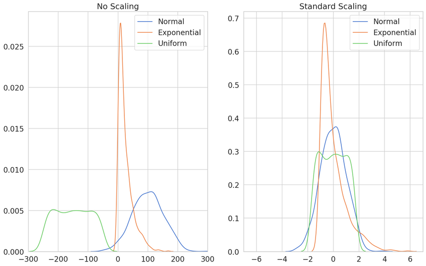
The resulting distributions overlap heavily. Also, their shape is much narrower.

This method “makes” a feature normally distributed. With outliers, your data will be scaled to a small interval.

Robust Scaling

This method is very similar to the Min-Max approach. Each feature is scaled with:

where $Q$ are quartiles. The Interquartile range makes this method robust to outliers (hence the name).

Let’s use the RobustScaler on our data:

1from sklearn.preprocessing import RobustScaler
2
3robust_scaled = RobustScaler().fit_transform(data)

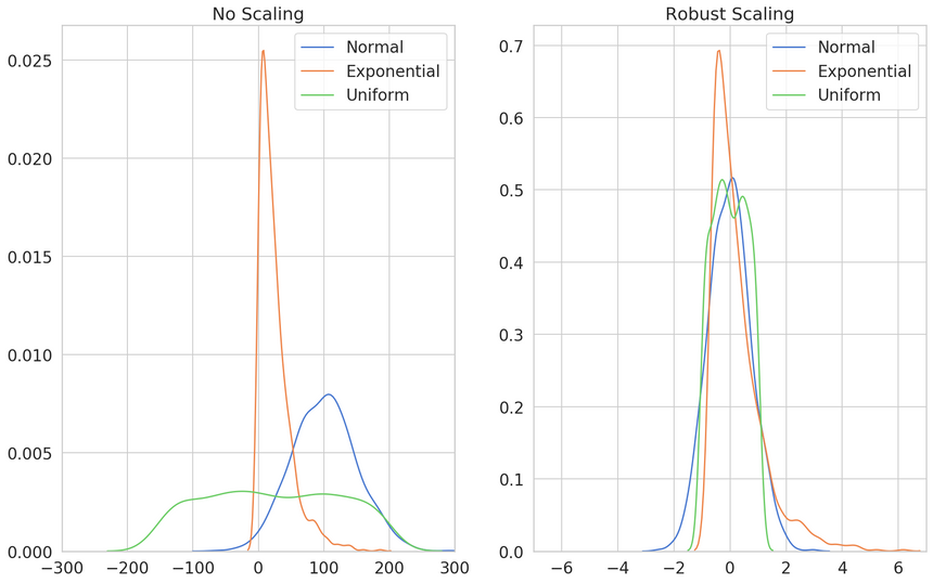
All distributions have most of their densities around 0 and a shape that is more or less the same.

Use this method when you have outliers and want to minimize their influence.

Scaling Methods Overview

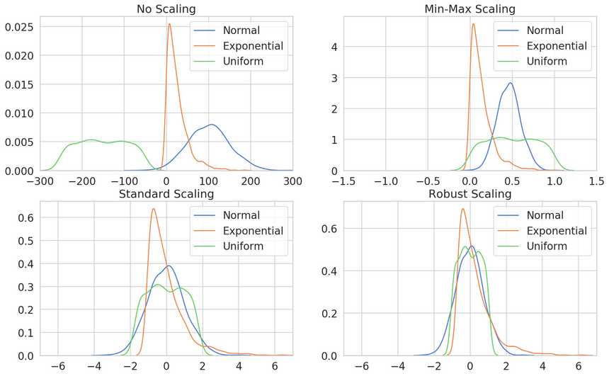
Here’s an overview of the scaled distributions compared to the non-scaled version:

Handling Categorical Data

Categorical variables (also known as nominal) are a set of enumerable values. They cannot be numerically organized or ranked. How can we use them in our Machine Learning algorithms?

Some algorithms, like decision trees, will work fine without any categorical data preprocessing. Unfortunatelly, that is the exception rather than the rule.

How can we encode the following property types?

1property_type =\
2    np.array(['House', 'Unit', 'Townhouse', 'House', 'Unit'])
3    .reshape(-1, 1)

Integer Encoding

Most Machine Learning algorithms require numeric-only data. One simple way to achieve that is to assing an unique value to each category.

We can use the OrdinalEncoder for that:

1from sklearn.preprocessing import OrdinalEncoder
2
3enc = OrdinalEncoder().fit(property_type)
4labels = enc.transform(property_type)
5labels.flatten()

1array([0., 2., 1., 0., 2.])

You can obtain the string representation of the categories like so:

1enc.inverse_transform(one_hots).flatten()

1array(['House', 'Unit', 'Townhouse', 'House', 'Unit'], dtype='<U9')

One-Hot Encoding

Unfortunatelly, the simple integer encoding makes the assumption that the categories can be ordered (ranked).

Sometimes, that assumption might be correct. When it is not, you can use one-hot encoding:

1from sklearn.preprocessing import OneHotEncoder
2
3enc = OneHotEncoder(sparse=False).fit(property_type)
4one_hots = enc.transform(property_type)
5one_hots

1array([[1., 0., 0.],
2       [0., 0., 1.],
3       [0., 1., 0.],
4       [1., 0., 0.],
5       [0., 0., 1.]])

Basically, one-hot encoding creates a vector of zeros for each row in our data with a one at the index (place) of the category.

This solves the ordering/ranking issue but introduces another one. Each categorical feature creates k (number of unique categories) new columns in our dataset, which are mostly zeros.

How Many Categories are Too Many for One-Hot Encoding?

With a vast amounts (number of rows) of data you might be able to get away with encoding lots of categorical features with a lot of categories.

Here are some ways to tackle the problem, when that is not possible:

• Drop insignificant features before encoding
• Drop columns with mostly zeros after encoding
• Create aggregate (larger) categories and one-hot encode them
• Encode them as integers and test your model performance

Adding New Features

Feature engineering refers to the process of augmenting your data (usually by adding features) using your (human) knowledge. This often improves the performance of Machine Learning algorithms.

Deep Learning has changed the feature engineering game when it comes to text and image data. Those algorithms learn intermediate representations of the data. In a way, they do automatic feature engineering.

When it comes to structured data (think data you get with SQL queries from your database), feature engineering might give you a lot of performance improvement.

How can we improve our datasets?

Turn Numbers into Categories

You already know how to convert categorical data to numbers. You can also turn ranges (bins) of numbers into categories. Let’s see an example:

1n_rooms = np.array([1, 2, 1, 4, 6, 7, 12, 20])

We’ll turn the number of rooms into three categories - small, medium and large:

1pd.cut(n_rooms, bins=[0, 3, 8, 100], labels=["small", "medium", "large"])

1[small, small, small, medium, medium, medium, large, large]
2Categories (3, object): [small < medium < large]

The cut() function from Pandas gives you a way to turn numbers into categories by specifying ranges and labels. Of course, you can use one-hot encoding on the new categories.

Extract Features from Dates

Dates in computers are represented as milliseconds since the Unix epoch - 00:00:00 UTC on 1 January 1970. You can use the raw numbers or extract some information from the dates. How can we do this with Pandas?

1dates = pd.Series(["1/04/2017", "2/04/2017", "3/04/2017"])

You can convert the string formatted dates into date objects with to_datetime(). This function works really well on a variety of formats. Let’s convert our dates:

1pd_dates = pd.to_datetime(dates)

One important feature we can get from the date values is the day of the week:

1pd_dates.dt.dayofweek

10    2
21    5
32    5
4dtype: int64

There you go, even more categorical data :)

Predicting Melbourne Housing Prices

Let’s use our new skills to do some data preprocessing on a real-world data. We’ll use the Melbourne Housing Market dataset available on Kaggle.

The Data

Here’s the description of the data:

This data was scraped from publicly available results posted every week from Domain.com.au, I’ve cleaned it as best I can, now it’s up to you to make data analysis magic. The dataset includes Address, Type of Real estate, Suburb, Method of Selling, Rooms, Price, Real Estate Agent, Date of Sale and distance from C.B.D.

Our task is to predict the sale price of the property based on a set of features. Let’s get the data using gdown:

1!gdown --id 1bIa7HOtpakl1Qzn6pmKCMAzrWjM08mfI --output melbourne_housing.csv

And load it into a Pandas dataframe:

1df = pd.read_csv('melbourne_housing.csv')
2df.shape

1(34857, 21)

We have almost 35k rows and 21 columns. Here are the features:

• Suburb
• Address
• Rooms
• Type - br - bedroom(s); h - house,cottage,villa, semi,terrace; u - unit, duplex; t - townhouse; dev site - development site; o res - other residential.
• Price - price in Australian dollars
• Method - S - property sold; SP - property sold prior; PI - property passed in; PN - sold prior not disclosed; SN - sold not disclosed; NB - no bid; VB - vendor bid; W - withdrawn prior to auction; SA - sold after auction; SS - sold after auction price not disclosed. N/A - price or highest bid not available.
• SellerG
• Date - date sold
• Distance
• Postcode
• Bedroom2
• Bathroom
• Car - number of carspots
• Landsize - land size in meters
• BuildingArea - building size in meters
• YearBuilt
• CouncilArea
• Lattitude
• Longtitude
• Regionname
• Propertycount - number of properties in the suburb

Let’s check for missing values:

1missing = df.isnull().sum()
2missing[missing > 0].sort_values(ascending=False)

1BuildingArea     21115
2YearBuilt        19306
3Landsize         11810
4Car               8728
5Bathroom          8226
6Bedroom2          8217
7Longtitude        7976
8Lattitude         7976
9Price             7610
10Propertycount        3
11Regionname           3
12CouncilArea          3
13Postcode             1
14Distance             1
15dtype: int64

We have a lot of those. For the purpose of this guide, we’re just going to drop all rows that contain missing values:

1df = df.dropna()

Predicting without Preprocessing

Let’s use the “raw” features to train a model and evaluate its performance. First, let’s split the data into training and test sets:

1X = df[[
2  'Rooms', 'Distance', 'Propertycount',
3  'Postcode', 'Lattitude', 'Longtitude'
4]]
5y = np.log1p(df.Price.values)
6
7X_train, X_test, y_train, y_test =\
8 train_test_split(X, y, test_size=0.2, random_state=RANDOM_SEED)

We’ll use the GradientBoostingRegressor and train it on our data:

1from sklearn.ensemble import GradientBoostingRegressor
2
3forest = GradientBoostingRegressor(
4  learning_rate=0.3, n_estimators=150, random_state=RANDOM_SEED
5).fit(X_train, y_train)
6
7forest.score(X_test, y_test)

10.7668970798114849

Good, now you have a baseline $R^2$ score on the raw data.

Preprocessing

Let’s start with something simple - extract the sale day of the week. We’ll add that to our dataset. You already know how to do this:

1df['Date'] = pd.to_datetime(df.Date)
2df['SaleDayOfWeek'] = df.Date.dt.dayofweek

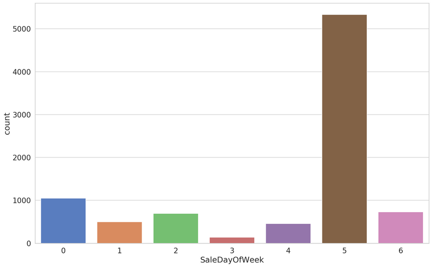
Saturday looks like a really important day for selling properties. Let’s have a look at the number of rooms:

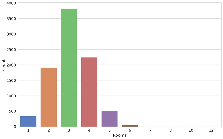
We can use the binning technique to create categories from the rooms:

1df['Size'] = pd.cut(
2  df.Rooms,
3  bins=[0, 2, 4, 100],
4  labels=["Small", "Medium", "Large"]
5)

Next, let’s drop some of the columns we’re not going to use:

1df = df.drop(['Address', 'Date'], axis=1)

Let’s create the training and test datasets:

1X = df.drop('Price', axis=1)
2y = np.log1p(df.Price.values)
3
4X_train, X_test, y_train, y_test =\
5 train_test_split(X, y, test_size=0.2, random_state=RANDOM_SEED)

The make_column_transformer() allows you to build an uber transformer™ composed of multiple transformers. Let’s use it on our data:

1from sklearn.compose import make_column_transformer
2
3transformer = make_column_transformer(
4    (RobustScaler(),
5      [
6        'Distance', 'Propertycount', 'Postcode',
7        'Lattitude', 'Longtitude', 'Rooms'
8      ]),
9    (OneHotEncoder(handle_unknown="ignore"),
10      ['Size', 'SaleDayOfWeek', 'Type', 'Method', 'Regionname']),
11    (OrdinalEncoder(
12        categories=[
13          X.CouncilArea.unique(),
14          X.SellerG.unique(),
15          X.Suburb.unique()],
16        dtype=np.int32
17      ), ['CouncilArea', 'SellerG', 'Suburb']
18    ),
19)

We’ll let the transformer learn only from the training data. That is vital since we don’t want our RobustScaler to leak information from the test set via the rescaled mean and variance.

Always: split the data into training and test set, then apply preprocessing

1transformer.fit(X_train)
2
3X_train = transformer.transform(X_train)
4X_test = transformer.transform(X_test)

Will your model perform better with the preprocessed data?

Predicting with Preprocessing

We’ll reuse the same model and train it on the preprocessed dataset:

1forest = GradientBoostingRegressor(
2  learning_rate=0.3,
3  n_estimators=150,
4  random_state=RANDOM_SEED
5).fit(X_train, y_train)
6forest.score(X_test, y_test)

10.8393772235062138

Considering that our baseline model was doing pretty well, you might be surprised by the improvement. It is definitely something.

Here’s a comparison of the predictions:

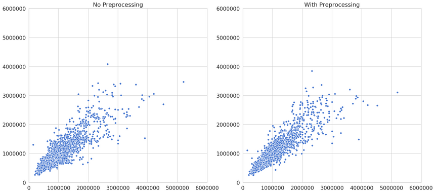
You can see that the predictions are looking much better (better predictions lie on the diagonal). Can you come up with more features/preprocessing to improve the $R^2$ score?

Conclusion

You’ve learned about some of the useful data preprocessing techniques. You’ve also applied what you’ve learned to a real-world dataset for predicting Melbourne Housing prices. Here’s an overview of the methods used:

• Feature Scaling
• Handling Categorical Data
• Feature Engineering

Do you use any other techniques to prepare your data?

Run the complete notebook in your browser

The complete project on GitHub

References

• Gradient descent in practice I: Feature Scaling
• Compare the effect of different scalers on data with outliers
• Feature Scaling
• Melbourne Housing Market