Heart Disease Prediction in TensorFlow 2 | TensorFlow for Hackers (Part II)
— Deep Learning, Neural Networks, TensorFlow, Python — 3 min read
Share
TL;DR Build and train a Deep Neural Network for binary classification in TensorFlow 2. Use the model to predict the presence of heart disease from patient data.
Machine Learning is used to solve real-world problems in many areas, already. Medicine is no exception. While controversial, multiple models have been proposed and used with some success. Some notable projects by Google and others:
Today, we’re going to take a look at one specific area - heart disease prediction.
About 610,000 people die of heart disease in the United States every year – that’s 1 in every 4 deaths. Heart disease is the leading cause of death for both men and women. More than half of the deaths due to heart disease in 2009 were in men. - Heart Disease Facts & Statistics | cdc.gov
Please note, the model presented here is very limited and in no way applicable for real-world situations. Our dataset is extremely small, conclusions made here are in no way generalizable. Heart disease prediction is a vastly more complex problem than depicted in this writing.
Complete source code in Google Colaboratory Notebook
Here is the plan:
- Explore patient data
- Data preprocessing
- Create your Neural Network in TensorFlow 2
- Train the model
- Predict heart disease from patient data
Patient Data
Our data comes from this dataset. It contains 303 patient records. Each record contains 14 attributes:
| Label | Description |
|---|---|
| age | age in years |
| sex | (1 = male; 0 = female) |
| cp | (1 = typical angina; 2 = atypical angina; 3 = non-anginal pain; 4 = asymptomatic) |
| trestbps | resting blood pressure (in mm Hg on admission to the hospital) |
| chol | serum cholestoral in mg/dl |
| fbs | (fasting blood sugar > 120 mg/dl) (1 = true; 0 = false) |
| restecg | resting electrocardiographic results |
| thalach | maximum heart rate achieved |
| exang | exercise induced angina (1 = yes; 0 = no) |
| oldpeak | ST depression induced by exercise relative to rest |
| slope | the slope of the peak exercise ST segment |
| ca | number of major vessels (0-3) colored by flourosopy |
| thal | (3 = normal; 6 = fixed defect; 7 = reversable defect) |
| target | (0 = no heart disease; 1 = heart disease presence) |
How many of the patient records indicate heart disease?
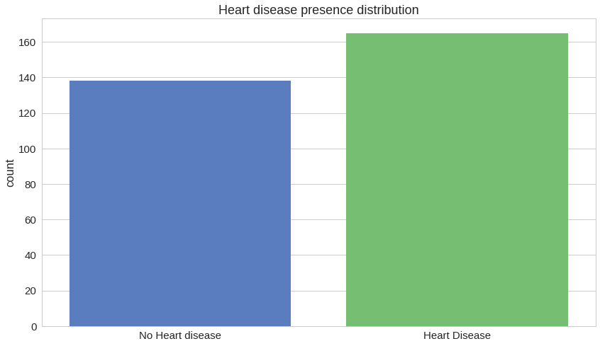
That looks like a pretty well-distributed dataset, considering the number of rows.
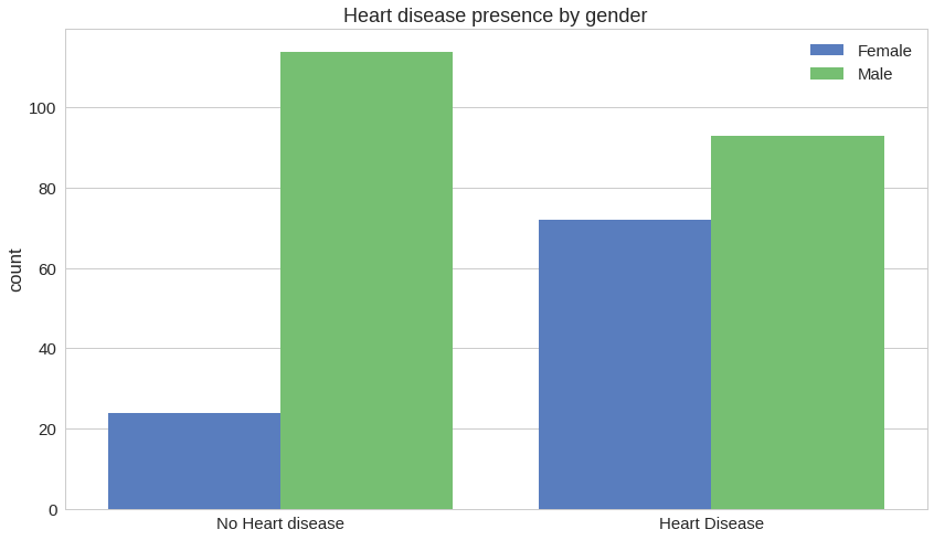
Let’s have a look at how heart disease affects different genders:
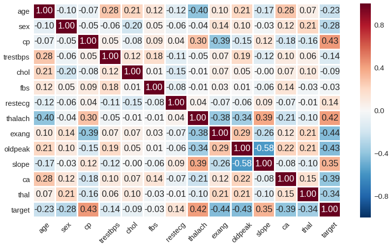
Here is a Pearson correlation heatmap between the features:
How disease presence is affected by thalach (“Maximum Heart Rate”) vs age:
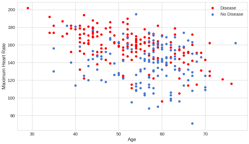
Looks like maximum heart rate can be very predictive for the presence of a disease, regardless of age.
How different types of chest pain affect the presence of heart disease:
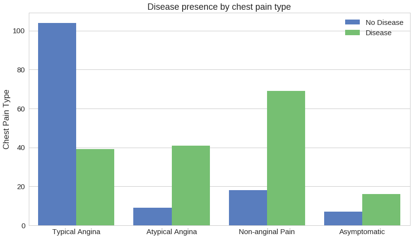
Having chest pain might not be indicative of heart disease.
Data Preprocessing
Our data contains a mixture of categorical and numerical data. Let’s use TensorFlow`s Feature Columns.
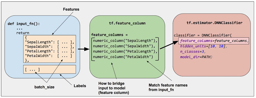 source: https://www.tensorflow.org/
Feature columns allow you to bridge/process the raw data in your dataset to fit your model input data requirements. Furthermore, you can separate the model building process from the data preprocessing. Let’s have a look:
1feature_columns = []23# numeric cols4for header in ['age', 'trestbps', 'chol', 'thalach', 'oldpeak', 'ca']:5 feature_columns.append(tf.feature_column.numeric_column(header))67# bucketized cols8age = tf.feature_column.numeric_column("age")9age_buckets = tf.feature_column.bucketized_column(age, boundaries=[18, 25, 30, 35, 40, 45, 50, 55, 60, 65])10feature_columns.append(age_buckets)1112# indicator cols13data["thal"] = data["thal"].apply(str)14thal = tf.feature_column.categorical_column_with_vocabulary_list(15 'thal', ['3', '6', '7'])16thal_one_hot = tf.feature_column.indicator_column(thal)17feature_columns.append(thal_one_hot)1819data["sex"] = data["sex"].apply(str)20sex = tf.feature_column.categorical_column_with_vocabulary_list(21 'sex', ['0', '1'])22sex_one_hot = tf.feature_column.indicator_column(sex)23feature_columns.append(sex_one_hot)2425data["cp"] = data["cp"].apply(str)26cp = tf.feature_column.categorical_column_with_vocabulary_list(27 'cp', ['0', '1', '2', '3'])28cp_one_hot = tf.feature_column.indicator_column(cp)29feature_columns.append(cp_one_hot)3031data["slope"] = data["slope"].apply(str)32slope = tf.feature_column.categorical_column_with_vocabulary_list(33 'slope', ['0', '1', '2'])34slope_one_hot = tf.feature_column.indicator_column(slope)35feature_columns.append(slope_one_hot)Apart from the numerical features, we’re putting patient age into discrete ranges (buckets). Furthermore, thal, sex, cp, and slope are categorical and we map them to such.
Next up, lets turn the pandas DataFrame into a TensorFlow Dataset:
1def create_dataset(dataframe, batch_size=32):2 dataframe = dataframe.copy()3 labels = dataframe.pop('target')4 return tf.data.Dataset.from_tensor_slices((dict(dataframe), labels)) \5 .shuffle(buffer_size=len(dataframe)) \6 .batch(batch_size)And split the data into training and testing:
1train, test = train_test_split(2 data,3 test_size=0.2,4 random_state=RANDOM_SEED5)67train_ds = create_dataset(train)8test_ds = create_dataset(test)The Model
Let’s build a binary classifier using Deep Neural Network in TensorFlow:
1model = tf.keras.models.Sequential([2 tf.keras.layers.DenseFeatures(feature_columns=feature_columns),3 tf.keras.layers.Dense(units=128, activation='relu'),4 tf.keras.layers.Dropout(rate=0.2),5 tf.keras.layers.Dense(units=128, activation='relu'),6 tf.keras.layers.Dense(units=2, activation='sigmoid')7])Our model uses the feature columns we’ve created in the preprocessing step. Note that, we’re no longer required to specify the input layer size.
We also use the Dropout layer between 2 dense layers. Our output layer contains 2 neurons, since we are building a binary classifier.
Training
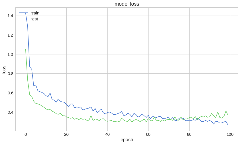
Our loss function is binary cross-entropy defined by:
−(ylog(p)+(1−y)log(1−p))where y is binary indicator if the predicted class is correct for the current observation and p is the predicted probability.
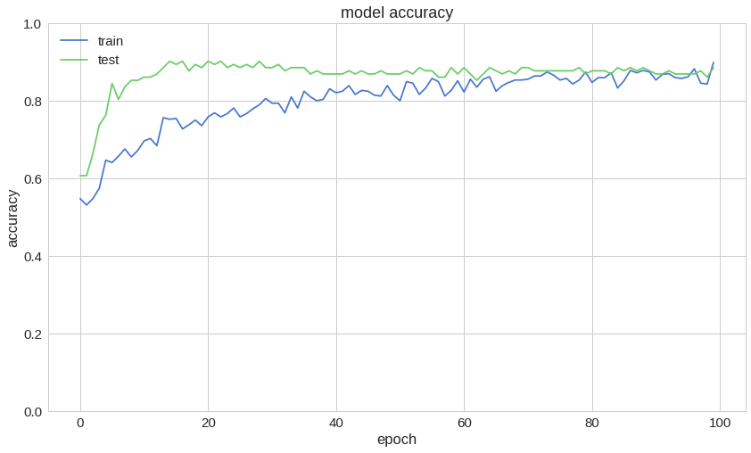
1model.compile(2 optimizer='adam',3 loss='binary_crossentropy',4 metrics=['accuracy']5)67history = model.fit(8 train_ds,9 validation_data=test_ds,10 epochs=100,11 use_multiprocessing=True12)Here is a sample of the training process:
1Epoch 95/10020s 42ms/step - loss: 0.3018 - accuracy: 0.8430 - val_loss: 0.4012 - val_accuracy: 0.86893Epoch 96/10040s 42ms/step - loss: 0.2882 - accuracy: 0.8547 - val_loss: 0.3436 - val_accuracy: 0.86895Epoch 97/10060s 42ms/step - loss: 0.2889 - accuracy: 0.8732 - val_loss: 0.3368 - val_accuracy: 0.86897Epoch 98/10080s 42ms/step - loss: 0.2964 - accuracy: 0.8386 - val_loss: 0.3537 - val_accuracy: 0.87709Epoch 99/100100s 43ms/step - loss: 0.3062 - accuracy: 0.8282 - val_loss: 0.4110 - val_accuracy: 0.860711Epoch 100/100120s 43ms/step - loss: 0.2685 - accuracy: 0.8821 - val_loss: 0.3669 - val_accuracy: 0.8852Accuracy on the test set:
1model.evaluate(test_ds)10s 24ms/step - loss: 0.3669 - accuracy: 0.88522[0.3669000566005707, 0.8852459]So, we have ~88% accuracy on the test set.
Predicting Heart Disease
Now that we have a model with some good accuracy on the test set, let’s try to predict heart disease based on the features in our dataset.
1predictions = tf.round(model.predict(test_ds)).numpy().flatten()Since we’re interested in making binary decisions, we’re taking the maximum probability of the output layer.
1print(classification_report(y_test.values, predictions))1precision recall f1-score support23 0 0.59 0.66 0.62 294 1 0.66 0.59 0.62 3256 micro avg 0.62 0.62 0.62 617 macro avg 0.62 0.62 0.62 618weighted avg 0.63 0.62 0.62 61Regardless of the accuracy, you can see that the precision, recall and f1-score of our model are not that high. Let’s take a look at the confusion matrix:
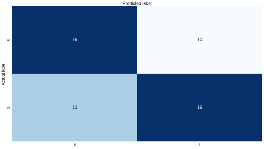
Our model looks a bit confused. Can you improve on it?
Conclusion
Complete source code in Google Colaboratory Notebook
You did it! You made a binary classifier using Deep Neural Network with TensorFlow and used it to predict heart disease from patient data.
Next, we’ll have a look at what TensorFlow 2 has in store for us, when applied to computer vision.
Share
Want to be a Machine Learning expert?
You'll never get spam from me