Curiousily

Human Activity Recognition using LSTMs on Android | TensorFlow for Hackers (Part VI)

03.06.2017 — Deep Learning, Neural Networks, TensorFlow, Python — 3 min read

Ever wondered how your smartphone, smartwatch or wristband knows when you’re walking, running or sitting? Well, your device probably has multiple sensors that give various information. GPS, audio (i.e. microphones), image (i.e. cameras), direction (i.e. compasses) and acceleration sensors are very common nowadays.

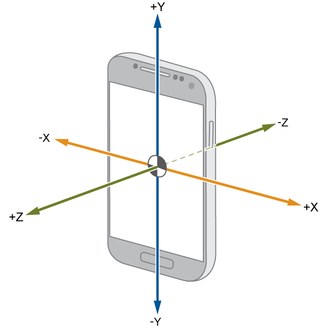source: Mathworks

We will use data collected from accelerometer sensors. Virtually every modern smartphone has a tri-axial accelerometer that measures acceleration in all three spatial dimensions. Additionally, accelerometers can detect device orientation.

In this part of the series, we will train an LSTM Neural Network (implemented in TensorFlow) for Human Activity Recognition (HAR) from accelerometer data. The trained model will be exported/saved and added to an Android app. We will learn how to use it for inference from Java.

The source code for this part is available (including the Android app) on GitHub.

The data

We will use data provided by the Wireless Sensor Data Mining (WISDM) Lab. It can be download from here. The dataset was collected in controlled, laboratory setting. The lab provides another dataset collected from real-world usage of a smartphone app. You’re free to use/explore it as well. Here’s a video that presents how a similar dataset was collected:

Our dataset contains 1,098,207 rows and 6 columns. There are no missing values. There are 6 activities that we’ll try to recognize: Walking, Jogging, Upstairs, Downstairs, Sitting, Standing. Let’s have a closer look at the data:

1import pandas as pd
2import numpy as np
3import pickle
4import matplotlib.pyplot as plt
5from scipy import stats
6import tensorflow as tf
7import seaborn as sns
8from pylab import rcParams
9from sklearn import metrics
10from sklearn.model_selection import train_test_split
11
12%matplotlib inline
13
14sns.set(style='whitegrid', palette='muted', font_scale=1.5)
15
16rcParams['figure.figsize'] = 14, 8
17
18RANDOM_SEED = 42

1columns = ['user','activity','timestamp', 'x-axis', 'y-axis', 'z-axis']
2df = pd.read_csv('data/WISDM_ar_v1.1_raw.txt', header = None, names = columns)
3df = df.dropna()

1df.head()

	user	activity	timestamp	x-axis	y-axis	z-axis
0	33	Jogging	49105962326000	-0.694638	12.680544	0.503953
1	33	Jogging	49106062271000	5.012288	11.264028	0.953424
2	33	Jogging	49106112167000	4.903325	10.882658	-0.081722
3	33	Jogging	49106222305000	-0.612916	18.496431	3.023717
4	33	Jogging	49106332290000	-1.184970	12.108489	7.205164

Exploration

The columns we will be most interested in are activity, x-axis, y-axis and z-axis. Let’s dive into the data:

1df['activity'].value_counts().plot(kind='bar', title='Training examples by activity type');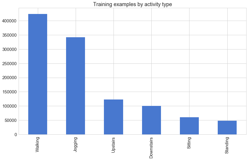

The columns we will be most interested in are activity, x-axis, y-axis and z-axis. Let’s dive into the data:

1df['user'].value_counts().plot(kind='bar', title='Training examples by user');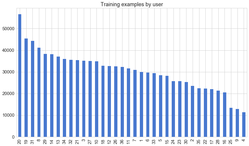

I wonder whether or not number 4 received the same paycheck as number 20. Now, for some accelerometer data:

1def plot_activity(activity, df):
2    data = df[df['activity'] == activity][['x-axis', 'y-axis', 'z-axis']][:200]
3    axis = data.plot(subplots=True, figsize=(16, 12),
4                     title=activity)
5    for ax in axis:
6        ax.legend(loc='lower left', bbox_to_anchor=(1.0, 0.5))

1plot_activity("Sitting", df)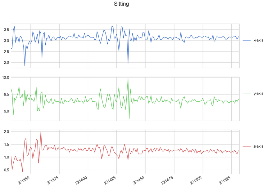

1plot_activity("Standing", df)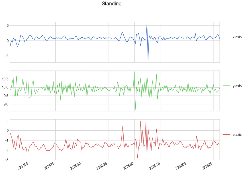

1plot_activity("Walking", df)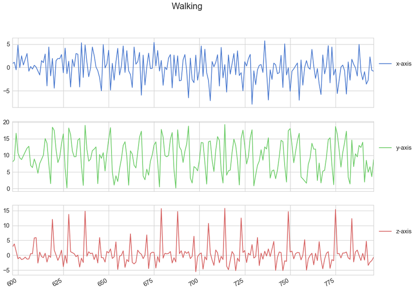

1plot_activity("Jogging", df)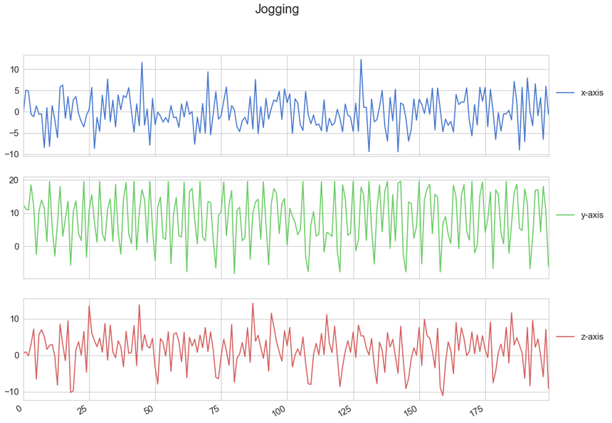

It seems reasonable to assume that this data might be used to train a model that can distinguish between the different kinds of activities. Well, at least the first 200 entries of each activity look that way.

Data preprocessing

Our LSTM (covered in the previous part of the series) model expects fixed-length sequences as training data. We’ll use a familiar method for generating these. Each generated sequence contains 200 training examples:

1N_TIME_STEPS = 200
2N_FEATURES = 3
3step = 20
4segments = []
5labels = []
6for i in range(0, len(df) - N_TIME_STEPS, step):
7    xs = df['x-axis'].values[i: i + N_TIME_STEPS]
8    ys = df['y-axis'].values[i: i + N_TIME_STEPS]
9    zs = df['z-axis'].values[i: i + N_TIME_STEPS]
10    label = stats.mode(df['activity'][i: i + N_TIME_STEPS])[0][0]
11    segments.append([xs, ys, zs])
12    labels.append(label)

1np.array(segments).shape

1(54901, 3, 200)

Our training dataset has drastically reduced size after the transformation. Note that we take the most common activity and assign it as a label for the sequence.

The shape of our tensor looks kinda strange. Let’s transform it into sequences of 200 rows, each containing x, y and z. Let’s apply a one-hot encoding to our labels, as well:

1reshaped_segments = np.asarray(segments, dtype= np.float32).reshape(-1, N_TIME_STEPS, N_FEATURES)
2labels = np.asarray(pd.get_dummies(labels), dtype = np.float32)

1reshaped_segments.shape

1(54901, 200, 3)

1labels[0]

1array([ 0.,  1.,  0.,  0.,  0.,  0.], dtype=float32)

Finally, let’s split the data into training and test (20%) set:

1X_train, X_test, y_train, y_test = train_test_split(
2        reshaped_segments, labels, test_size=0.2, random_state=RANDOM_SEED)

Building the model

Our model contains 2 fully-connected and 2 LSTM layers (stacked on each other) with 64 units each:

1N_CLASSES = 6
2N_HIDDEN_UNITS = 64

1def create_LSTM_model(inputs):
2    W = {
3        'hidden': tf.Variable(tf.random_normal([N_FEATURES, N_HIDDEN_UNITS])),
4        'output': tf.Variable(tf.random_normal([N_HIDDEN_UNITS, N_CLASSES]))
5    }
6    biases = {
7        'hidden': tf.Variable(tf.random_normal([N_HIDDEN_UNITS], mean=1.0)),
8        'output': tf.Variable(tf.random_normal([N_CLASSES]))
9    }
10
11    X = tf.transpose(inputs, [1, 0, 2])
12    X = tf.reshape(X, [-1, N_FEATURES])
13    hidden = tf.nn.relu(tf.matmul(X, W['hidden']) + biases['hidden'])
14    hidden = tf.split(hidden, N_TIME_STEPS, 0)
15
16    # Stack 2 LSTM layers
17    lstm_layers = [tf.contrib.rnn.BasicLSTMCell(N_HIDDEN_UNITS, forget_bias=1.0) for _ in range(2)]
18    lstm_layers = tf.contrib.rnn.MultiRNNCell(lstm_layers)
19
20    outputs, _ = tf.contrib.rnn.static_rnn(lstm_layers, hidden, dtype=tf.float32)
21
22    # Get output for the last time step
23    lstm_last_output = outputs[-1]
24
25    return tf.matmul(lstm_last_output, W['output']) + biases['output']

Now, let create placeholders for our model:

1tf.reset_default_graph()
2
3X = tf.placeholder(tf.float32, [None, N_TIME_STEPS, N_FEATURES], name="input")
4Y = tf.placeholder(tf.float32, [None, N_CLASSES])

Note that we named the input tensor, that will be useful when using the model from Android. Creating the model:

1pred_Y = create_LSTM_model(X)
2
3pred_softmax = tf.nn.softmax(pred_Y, name="y_")

Again, we must properly name the tensor from which we will obtain predictions. We will use L2 regularization and that must be noted in our loss op:

1L2_LOSS = 0.0015
2
3l2 = L2_LOSS * \
4    sum(tf.nn.l2_loss(tf_var) for tf_var in tf.trainable_variables())
5
6loss = tf.reduce_mean(tf.nn.softmax_cross_entropy_with_logits(logits = pred_Y, labels = Y)) + l2

Finally, let’s define optimizer and accuracy ops:

1LEARNING_RATE = 0.0025
2
3optimizer = tf.train.AdamOptimizer(learning_rate=LEARNING_RATE).minimize(loss)
4
5correct_pred = tf.equal(tf.argmax(pred_softmax, 1), tf.argmax(Y, 1))
6accuracy = tf.reduce_mean(tf.cast(correct_pred, dtype=tf.float32))

Training

The training part contains a lot of TensorFlow boilerplate. We will train our model for 50 epochs and keep track of accuracy and error:

1N_EPOCHS = 50
2BATCH_SIZE = 1024

1saver = tf.train.Saver()
2
3history = dict(train_loss=[],
4                     train_acc=[],
5                     test_loss=[],
6                     test_acc=[])
7
8sess=tf.InteractiveSession()
9sess.run(tf.global_variables_initializer())
10
11train_count = len(X_train)
12
13for i in range(1, N_EPOCHS + 1):
14    for start, end in zip(range(0, train_count, BATCH_SIZE),
15                          range(BATCH_SIZE, train_count + 1,BATCH_SIZE)):
16        sess.run(optimizer, feed_dict={X: X_train[start:end],
17                                       Y: y_train[start:end]})
18
19    _, acc_train, loss_train = sess.run([pred_softmax, accuracy, loss], feed_dict={
20                                            X: X_train, Y: y_train})
21
22    _, acc_test, loss_test = sess.run([pred_softmax, accuracy, loss], feed_dict={
23                                            X: X_test, Y: y_test})
24
25    history['train_loss'].append(loss_train)
26    history['train_acc'].append(acc_train)
27    history['test_loss'].append(loss_test)
28    history['test_acc'].append(acc_test)
29
30    if i != 1 and i % 10 != 0:
31        continue
32
33    print(f'epoch: {i} test accuracy: {acc_test} loss: {loss_test}')
34
35predictions, acc_final, loss_final = sess.run([pred_softmax, accuracy, loss], feed_dict={X: X_test, Y: y_test})
36
37print()
38print(f'final results: accuracy: {acc_final} loss: {loss_final}')

1epoch: 1 test accuracy: 0.7736998796463013 loss: 1.2773654460906982
2epoch: 10 test accuracy: 0.9388942122459412 loss: 0.5612533092498779
3epoch: 20 test accuracy: 0.9574717283248901 loss: 0.3916512429714203
4epoch: 30 test accuracy: 0.9693103432655334 loss: 0.2935260236263275
5epoch: 40 test accuracy: 0.9747744202613831 loss: 0.2502188980579376

Whew, that was a lot of training. Do you feel thirsty? Let’s store our precious model to disk:

1pickle.dump(predictions, open("predictions.p", "wb"))
2pickle.dump(history, open("history.p", "wb"))
3tf.train.write_graph(sess.graph_def, '.', '/media/old-tf-hackers-6/checkpoint/har.pbtxt')
4saver.save(sess, save_path = "/media/old-tf-hackers-6/checkpoint/har.ckpt")
5sess.close()

And loading it back:

1history = pickle.load(open("history.p", "rb"))
2predictions = pickle.load(open("predictions.p", "rb"))

Evaluation

1plt.figure(figsize=(12, 8))
2
3plt.plot(np.array(history['train_loss']), "r--", label="Train loss")
4plt.plot(np.array(history['train_acc']), "g--", label="Train accuracy")
5
6plt.plot(np.array(history['test_loss']), "r-", label="Test loss")
7plt.plot(np.array(history['test_acc']), "g-", label="Test accuracy")
8
9plt.title("Training session's progress over iterations")
10plt.legend(loc='upper right', shadow=True)
11plt.ylabel('Training Progress (Loss or Accuracy values)')
12plt.xlabel('Training Epoch')
13plt.ylim(0)
14
15plt.show()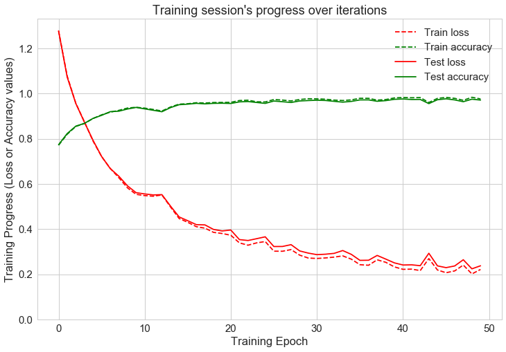

Our model seems to learn well with accuracy reaching above 97% and loss hovering at around 0.2. Let’s have a look at the confusion matrix for the model’s predictions:

1LABELS = ['Downstairs', 'Jogging', 'Sitting', 'Standing', 'Upstairs', 'Walking']

1max_test = np.argmax(y_test, axis=1)
2max_predictions = np.argmax(predictions, axis=1)
3confusion_matrix = metrics.confusion_matrix(max_test, max_predictions)
4
5plt.figure(figsize=(16, 14))
6sns.heatmap(confusion_matrix, xticklabels=LABELS, yticklabels=LABELS, annot=True, fmt="d");
7plt.title("Confusion matrix")
8plt.ylabel('True label')
9plt.xlabel('Predicted label')
10plt.show();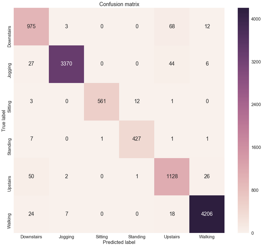

Again, it looks like our model performs real good. Some notable exceptions include the misclassification of Upstairs for Downstairs and vice versa. Jogging seems to fail us from time to time as well!

Exporting the model

Now that most of the hard work is done we must export our model in a way that TensorFlow for Android will understand it:

1from tensorflow.python.tools import freeze_graph
2
3MODEL_NAME = 'har'
4
5input_graph_path = 'checkpoint/' + MODEL_NAME+'.pbtxt'
6checkpoint_path = '/media/old-tf-hackers-6/checkpoint/' +MODEL_NAME+'.ckpt'
7restore_op_name = "save/restore_all"
8filename_tensor_name = "save/Const:0"
9output_frozen_graph_name = 'frozen_'+MODEL_NAME+'.pb'
10
11freeze_graph.freeze_graph(input_graph_path, input_saver="",
12                          input_binary=False, input_checkpoint=checkpoint_path,
13                          output_node_names="y_", restore_op_name="save/restore_all",
14                          filename_tensor_name="save/Const:0",
15                          output_graph=output_frozen_graph_name, clear_devices=True, initializer_nodes="")

1INFO:tensorflow:Restoring parameters from /media/old-tf-hackers-6/checkpoint/har.ckpt
2INFO:tensorflow:Froze 8 variables.
3Converted 8 variables to const ops.
46862 ops in the final graph.

A sample app that uses the exported model can be found on GitHub. It is based heavily based on the Activity Recognition app by Aaqib Saeed. Our app uses the text-to-speech Android API to tell you what the model predicts at some interval and includes our pre-trained model.

The most notable parts of the Java code include defining our input and output dimensions and names:

1String INPUT_NODE = "inputs";
2String[] OUTPUT_NODES = {"y_"};
3String OUTPUT_NODE = "y_";
4long[] INPUT_SIZE = {1, 200, 3};
5int OUTPUT_SIZE = 6;

Creating the TensorFlowInferenceInterface:

1inferenceInterface = new TensorFlowInferenceInterface(context.getAssets(), MODEL_FILE);

And making the predictions:

1public float[] predictProbabilities(float[] data) {
2    float[] result = new float[OUTPUT_SIZE];
3    inferenceInterface.feed(INPUT_NODE, data, INPUT_SIZE);
4    inferenceInterface.run(OUTPUT_NODES);
5    inferenceInterface.fetch(OUTPUT_NODE, result);
6
7    //Downstairs    Jogging   Sitting   Standing    Upstairs    Walking
8    return result;
9}

The result is a float array that contains the probability for each possible activity, according to our model.

Conclusion

We’ve built an LSTM model that can predict human activity from 200 time-step sequence with over 97% accuracy on the test set. The model was exported and used in an Android app. I had a lot of fun testing it on my phone, but it seems like more fine tuning (or changing the dataset) is required. Did you try the app? Can you improve it?

The source code for this part is available (including the Android app) on GitHub.

References

Want to be a Machine Learning expert?

Join the weekly newsletter on Data Science, Deep Learning and Machine Learning in your inbox, curated by me! Chosen by 10,000+ Machine Learning practitioners. (There might be some exclusive content, too!)

You'll never get spam from me

Hacker's Guide to Neural Networks in JavaScript

Build Machine Learning models (especially Deep Neural Networks) that you can easily integrate with existing or new web apps. Think of your ReactJs, Vue, or Angular app enhanced with the power of Machine Learning models.

Get SH*T Done with PyTorch

Learn how to solve real-world problems with Deep Learning models (NLP, Computer Vision, and Time Series). Go from prototyping to deployment with PyTorch and Python!

Hacker's Guide to Machine Learning with Python

This book brings the fundamentals of Machine Learning to you, using tools and techniques used to solve real-world problems in Computer Vision, Natural Language Processing, and Time Series analysis. The skills taught in this book will lay the foundation for you to advance your journey to Machine Learning Mastery!

Hands-On Machine Learning from Scratch

This book will guide you on your journey to deeper Machine Learning understanding by developing algorithms in Python from scratch! Learn why and when Machine learning is the right tool for the job and how to improve low performing models!