Movie review sentiment analysis with Naive Bayes | Machine Learning from Scratch (Part V)
— Machine Learning, Statistics, Sentiment Analysis, Text Classification — 5 min read
Share
TL;DR Build Naive Bayes text classification model using Python from Scratch. Use the model to classify IMDB movie reviews as positive or negative.
Textual data dominates our world from the tweets you read to the timeless writings of Seneca. And while we’re consuming images (looking at you Instagram) and videos at increasing rates, you still read Google search results multiple times per daily.
One frequently recurring problem with text data is Sentiment analysis (classification). Imagine you’re a big sugar + water beverage company. You want to know what people think of your products. You’ll search for texts with some tags, logos or names. You can then use Sentiment analysis to figure out if the opinions are positive or negative. Of course, you’ll send the negative ones to your highly underpaid support center in India to sort things out.
Here, we’ll build a generic text classifier that puts movie review texts into one of two categories - negative or positive sentiment. We’re going to have a brief look at the Bayes theorem and relax its requirements using the Naive assumption.
Complete source code in Google Colaboratory Notebook
Dealing with Text
Computers don’t understand text data, though they do well with numbers. Natural Language Processing (NLP) offers a set of approaches to solve text-related problems and represent text as numbers. While NLP is a vast field, we’ll use some simple preprocessing techniques and Bag of Words model.
The Data
Our data comes from a Kaggle challenge - “Bag of Words Meets Bags of Popcorn”.
We have 25,000 movie reviews from IMDB labeled as positive or negative. You might know that IMDB ratings are in the 0-10 range. An additional preprocessing step, done by the dataset authors, converts the rating to binary sentiment (<5 - negative ). Of course, a single movie can have multiple reviews, but no more than 30.
Reading the reviews
Let’s load the training and test data in Pandas data frames:
1train = pd.read_csv("imdb_review_train.tsv", delimiter="\t")2test = pd.read_csv("imdb_review_test.tsv", delimiter="\t")Exploration
Let’s get a feel for our data. Here are the first 5 rows of the training data:
| id | sentiment | review |
|---|---|---|
| 5814_8 | 1 | With all this stuff going down at the moment w… |
| 2381_9 | 1 | \The Classic War of the Worlds\” by Timothy Hi… |
| 7759_3 | 0 | The film starts with a manager (Nicholas Bell)… |
| 3630_4 | 0 | It must be assumed that those who praised this… |
| 9495_8 | 1 | Superbly trashy and wondrously unpretentious 8… |
We’re going to focus on the sentiment and review columns. The id column is combining the movie id with a unique number of a review. This might be a piece of important information in real-world scenarios, but we’re going to keep it simple.

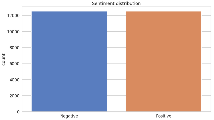
Both positive and negative sentiments have an equal presence. No need for additional gimmicks to fix that!
Here are the most common words in the training dataset reviews:

Hmm, that br looks weird, right?
Cleaning
Real-world text data is really messy. It can contain excessive punctuation, HTML tags (including that br), multiple spaces, etc. We’ll try to remove/normalize most of it.
Most of the cleaning we’ll do using Regular Expressions, but we’ll use two libraries to handle HTML tags (surprisingly hard to remove) and removing common (stop) words:
1def clean(self, text):2 no_html = BeautifulSoup(text).get_text()3 clean = re.sub("[^a-z\s]+", " ", no_html, flags=re.IGNORECASE)4 return re.sub("(\s+)", " ", clean)First, we use BeautifulSoup to remove HTML tags from our text. Second, we remove anything that is not a letter or space (note the ignoring of uppercase characters). Finally, we replace excessive spacing with a single one.
Tokenization
Now that our reviews are “clean”, we can further prepare them for our Bag of Words model. Let’s them to lowercase letters and split them into individual words. This process is known as tokenization:
1def tokenize(self, text):2 clean = self.clean(text).lower()3 stopwords_en = stopwords.words("english")4 return [w for w in re.split("\W+", clean) if not w in stopwords_en]The last step of our pre-processing is to remove stop words using those defined in the NLTK library. Stop words are usually frequently occurring words that might not significantly affect the meaning of the text. Some examples in English are: “is”, “the”, “and”.
An additional benefit of removing stop words is speeding up our models since we’re removing the amount of train/test data. However, in real-world scenarios, you should think about whether removing stop words can be justified.
We’ll place our clean and tokenize function in a class called Tokenizer.
Naive Bayes
Naive Bayes models are probabilistic classifiers that use the Bayes theorem and make a strong assumption that the features of the data are independent. For our case, this means that each word is independent of others.
Intuitively, this might sound like a dumb idea. You know that (even from reading) the prev word(s) influence the current and next ones. However, the assumption simplifies the math and works really well in practice!
The Bayes theorem is defined as:
P(A∣B)=P(B)P(B∣A)P(A)where A and B are some events and P(.) is a probability.
This equation gives us the conditional probability of event A occurring given B has happened. In order to find this, we need to calculate the probability of B happening given A has happened and multiply that by the probability of A (known as Prior) happening. All of this is divided by the probability of B happening on its own.
The naive assumption allows us to reformulate the Bayes theorem for our example as:
P(Sentiment∣w1,…,wn)=P(w1,…,wn)P(Sentiment)i=1∏nP(wi∣Sentiment)We don’t really care about probabilities. We only want to know whether a given text has a positive or negative sentiment. We can skip the denominator entirely since it just scales the numerator:
P(Sentiment∣w1,…,wn)∝P(Sentiment)i=1∏nP(wi∣Sentiment)To choose the sentiment, we’ll compare the scores for each sentiment and pick the one with a higher score.
Implementing Multinomial Naive Bayes
As you might’ve guessed by now, we’re classifying text into one of two groups/categories - positive and negative sentiment.
Multinomial Naive Bayes allows us to represent the features of the model as frequencies of their occurrences (how often some word is present in our review). In other words, it tells us that the probability distributions we’re using are multinomial.
Note on numerical stability
Our model relies on multiplying many probabilities. Those might become increasingly small and our computer might round them down to zero. To combat this, we’re going to use log probability by taking log of each side in our equation:
logP(Sentiment∣w1,…,wn)=logP(Sentiment)+logi=1∏nP(wi∣Sentiment)Note that we can still use the highest score of our model to predict the sentiment since log is monotonic.
Building our model
Finally, time to implement our model in Python. Let’s start by defining some variables and group the data by class, so our training code is a bit tidier:
1def fit(self, X, y):2 self.n_class_items = {}3 self.log_class_priors = {}4 self.word_counts = {}5 self.vocab = set()67 n = len(X)8 grouped_data = self.group_by_class(X, y)9 ...We’re going to implement a generic text classifier that doesn’t assume the number of classes. You can use it for news category prediction, sentiment analysis, email spam detection, etc.
For each class, we’ll find the number of examples in it and the log probability (prior). We’ll also record the number of occurrences of each word and create a vocabulary - set of all words we’ve seen in the training data:
1...2 for c, data in grouped_data.items():3 self.n_class_items[c] = len(data)4 self.log_class_priors[c] = math.log(self.n_class_items[c] / n)5 self.word_counts[c] = defaultdict(lambda: 0)67 for text in data:8 counts = Counter(self.tokenizer.tokenize(text))9 for word, count in counts.items():10 if word not in self.vocab:11 self.vocab.add(word)1213 self.word_counts[c][word] += countNote that we use our Tokenizer and the built-in class Counter to convert a review to a bag of words.
In case you’re interested, here’s how group_by_class works:
1def group_by_class(self, X, y):2 data = dict()3 for c in self.classes:4 data[c] = X[np.where(y == c)]5 return dataMaking predictions
In order to predict sentiment from text data, we’ll use our class priors and vocabulary:
1def predict(self, X):2 result = []3 for text in X:45 class_scores = {c: self.log_class_priors[c] for c in self.classes}6 words = set(self.tokenizer.tokenize(text))78 for word in words:9 if word not in self.vocab: continue1011 for c in self.classes:1213 log_w_given_c = self.laplace_smoothing(word, c)14 class_scores[c] += log_w_given_c1516 result.append(max(class_scores, key=class_scores.get))1718 return resultFor each review, we use the log priors for positive and negative sentiment and tokenize the text. For each word, we check if it is in the vocabulary and skip it if it is not. Then we calculate the log probability of this word for each class. We add the class scores and pick the class with a max score as our prediction.
Laplace smoothing
Note that log(0) is undefined (and no, we’re not using JavaScript here). It is entirely possible for a word in our vocabulary to be present in one class but not another - the probability of finding this word in that class will be 0! We can use Laplace smoothing to fix this problem. We’ll simply add 1 to the numerator but also add the size of our vocabulary to the denominator:
1def laplace_smoothing(self, word, text_class):2 num = self.word_counts[text_class][word] + 13 denom = self.n_class_items[text_class] + len(self.vocab)4 return math.log(num / denom)Predicting sentiment
Now that your model can be trained and make predictions, let’s use it to predict sentiment from movie reviews.
Data preparation
As discussed previously, we’ll use only the review and sentiment columns from the training data. Let split it for training and testing:
1X = train['review'].values2y = train['sentiment'].values34X_train, X_test, y_train, y_test = train_test_split(X, y, test_size=0.2, random_state=RANDOM_SEED)Evaluation
We’ll pack our fit and predict functions into a class called MultinomialNaiveBayes. Let’s use it:
1MNB = MultinomialNaiveBayes(2 classes=np.unique(y),3 tokenizer=Tokenizer()4).fit(X_train, y_train)Our classifier takes a list of possible classes and a Tokenizer as parameters. Also, the API is quite nice (thanks scikit-learn!)
1y_hat = MNB.predict(X_test)2accuracy_score(y_test, y_hat)10.8556This looks nice. We got an accuracy of ~86% on the test set.
Here is the classification report:
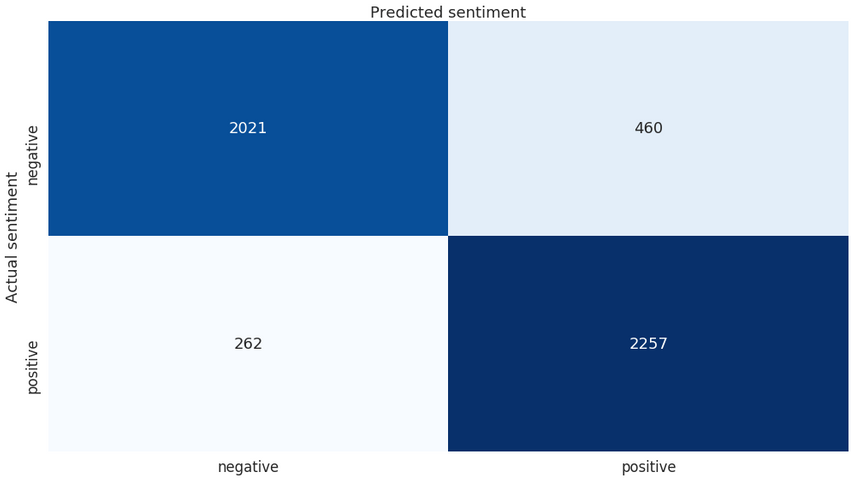
1precision recall f1-score support23 0 0.89 0.81 0.85 24814 1 0.83 0.90 0.86 251956 accuracy 0.86 50007 macro avg 0.86 0.86 0.86 50008weighted avg 0.86 0.86 0.86 5000And the confusion matrix:

Overall, our classifier does pretty well for himself. Submit the predictions to Kaggle and find out what place you’ll get on the leaderboard.
Conclusion
Well done! You just built a Multinomial Naive Bayes classifier that does pretty well on sentiment prediction. You also learned about Bayes theorem, text processing, and Laplace smoothing! Will another flavor of the Naive Bayes classifier perform better?
Complete source code in Google Colaboratory Notebook
Next up, you’ll build a recommender system from scratch!
Share
Want to be a Machine Learning expert?
You'll never get spam from me