TL;DR Learn how to prepare a custom dataset for object detection and detect vehicle plates. Use transfer learning to finetune the model and make predictions on test images.

Detecting objects in images and video is a hot research topic and really useful in practice. The advancement in Computer Vision (CV) and Deep Learning (DL) made training and running object detectors possible for practitioners of all scale. Modern object detectors are both fast and much more accurate (actually, usefully accurate).

This guide shows you how to fine-tune a pre-trained Neural Network on a large Object Detection dataset. We’ll learn how to detect vehicle plates from raw pixels. Spoiler alert, the results are not bad at all!

You’ll learn how to prepare a custom dataset and use a library for object detection based on TensorFlow and Keras. Along the way, we’ll have a deeper look at what Object Detection is and what models are used for it.

Here’s what will do:

• Understand Object Detection
• RetinaNet
• Prepare the Dataset
• Train a Model to Detect Vehicle Plates

Run the complete notebook in your browser

The complete project on GitHub

Object Detection

Object detection methods try to find the best bounding boxes around objects in images and videos. It has a wide array of practical applications - face recognition, surveillance, tracking objects, and more.

A lot of classical approaches have tried to find fast and accurate solutions to the problem. Sliding windows for object localization and image pyramids for detection at different scales are one of the most used ones. Those methods were slow, error-prone, and not able to handle object scales very well.

Deep Learning changed the field so much that it is now relatively easy for the practitioner to train models on small-ish datasets and achieve high accuracy and speed.

Usually, the result of object detection contains three elements:

• list of bounding boxes with coordinates
• the category/label for each bounding box
• the confidence score (0 to 1) for each bounding box and label

How can you evaluate the performance of object detection models?

Evaluating Object Detection

The most common measurement you’ll come around when looking at object detection performance is Intersection over Union (IoU). This metric can be evaluated independently of the algorithm/model used.

The IoU is a ratio given by the following equation:

IoU allows you to evaluate how well two bounding boxes overlap. In practice, you would use the annotated (true) bounding box, and the detected/predicted one. A value close to 1 indicates a very good overlap while getting closer to 0 gives you almost no overlap.

Getting IoU of 1 is very unlikely in practice, so don’t be too harsh on your model.

Mean Average Precision (mAP)

Reading papers and leaderboards on Object Detection will inevitably lead you to an mAP value report. Typically, you’ll see something like mAP@0.5 indicating that object detection is considered correct only when this value is greater than 0.5.

The value is derived by averaging the precision of each class in the dataset. We can get the average precision for a single class by computing the IoU for every example in the class and divide by the number of class examples. Finally, we can get mAP by dividing by the number of classes.

RetinaNet

RetinaNet, presented by Facebook AI Research in Focal Loss for Dense Object Detection (2017), is an object detector architecture that became very popular and widely used in practice. Why is RetinaNet so special?

RetinaNet is a one-stage detector. The most successful object detectors up to this point were operating on two stages (R-CNNs). The first stage involves selecting a set of regions (candidates) that might contain objects of interest. The second stage applies a classifier to the proposals.

One stage detectors (like RetinaNet) skip the region selection steps and runs detection over a lot of possible locations. This is faster and simpler but might reduce the overall prediction performance of the model.

RetinaNet is built on top of two crucial concepts - Focal Loss and Featurized Image Pyramid:

• Focal Loss is designed to mitigate the issue of extreme imbalance between background and foreground with objects of interest. It assigns more weight on hard, easily misclassified examples and small weight to easier ones.

• The Featurized Image Pyramid is the vision component of RetinaNet. It allows for object detection at different scales by stacking multiple convolutional layers.

Keras Implementation

Let’s get real. RetinaNet is not a SOTA model for object detection. Not by a long shot. However, well maintained, bug-free, and easy to use implementation of a good-enough model can give you a good estimate of how well you can solve your problem. In practice, you want a good-enough solution to your problem, and you (or your manager) wants it yesterday.

Keras RetinaNet is a well maintained and documented implementation of RetinaNet. Go and have a look at the Readme to get a feel of what is capable of. It comes with a lot of pre-trained models and an easy way to train on custom datasets.

Preparing the Dataset

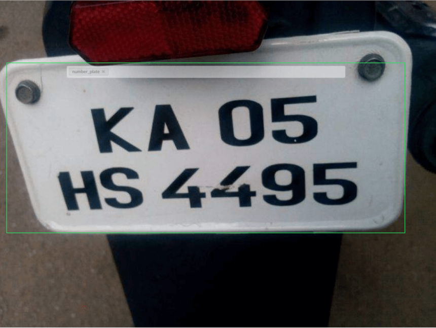
The task we’re going to work on is vehicle number plate detection from raw images. Our data is hosted on Kaggle and contains an annotation file with links to the images. Here’s a sample annotation:

1{
2  "content": "http://com.dataturks.a96-i23.open.s3.amazonaws.com/2c9fafb0646e9cf9016473f1a561002a/77d1f81a-bee6-487c-aff2-0efa31a9925c____bd7f7862-d727-11e7-ad30-e18a56154311.jpg",
3  "annotation": [
4    {
5      "label": [
6        "number_plate"
7      ],
8      "notes": null,
9      "points": [
10        {
11          "x": 0.7220843672456576,
12          "y": 0.5879828326180258
13        },
14        {
15          "x": 0.8684863523573201,
16          "y": 0.6888412017167382
17        }
18      ],
19      "imageWidth": 806,
20      "imageHeight": 466
21    }
22  ],
23  "extras": null
24}

This will require some processing to turn those xs and ys into proper image positions. Let’s start with downloading the JSON file:

1!gdown --id 1mTtB8GTWs74Yeqm0KMExGJZh1eDbzUlT --output indian_number_plates.json

We can use Pandas to read the JSON into a DataFrame:

1plates_df = pd.read_json('indian_number_plates.json', lines=True)

Next, we’ll download the images in a directory and create an annotation file for our training data in the format (expected by Keras RetinaNet):

1path/to/image.jpg,x1,y1,x2,y2,class_name

Let’s start by creating the directory:

1os.makedirs("number_plates", exist_ok=True)

We can unify the download and the creation of annotation file like so:

1dataset = dict()
2dataset["image_name"] = list()
3dataset["top_x"] = list()
4dataset["top_y"] = list()
5dataset["bottom_x"] = list()
6dataset["bottom_y"] = list()
7dataset["class_name"] = list()
8
9counter = 0
10for index, row in plates_df.iterrows():
11    img = urllib.request.urlopen(row["content"])
12    img = Image.open(img)
13    img = img.convert('RGB')
14    img.save(f'number_plates/licensed_car_{counter}.jpeg', "JPEG")
15
16    dataset["image_name"].append(
17      f'number_plates/licensed_car_{counter}.jpeg'
18    )
19
20    data = row["annotation"]
21
22    width = data[0]["imageWidth"]
23    height = data[0]["imageHeight"]
24
25    dataset["top_x"].append(
26      int(round(data[0]["points"][0]["x"] * width))
27    )
28    dataset["top_y"].append(
29      int(round(data[0]["points"][0]["y"] * height))
30    )
31    dataset["bottom_x"].append(
32      int(round(data[0]["points"][1]["x"] * width))
33    )
34    dataset["bottom_y"].append(
35      int(round(data[0]["points"][1]["y"] * height))
36    )
37    dataset["class_name"].append("license_plate")
38
39    counter += 1
40print("Downloaded {} car images.".format(counter))

We can use the dict to create a Pandas DataFrame:

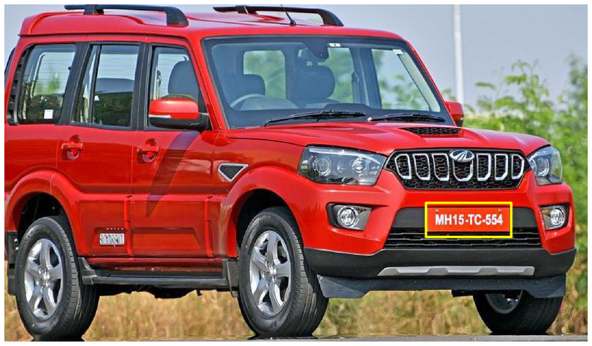
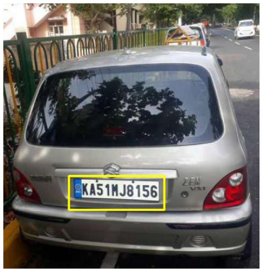
1df = pd.DataFrame(dataset)

Let’s get a look at some images of vehicle plates:

Preprocessing

We’ve already done a fair bit of preprocessing. A bit more is needed to convert the data into the format that Keras Retina understands:

1path/to/image.jpg,x1,y1,x2,y2,class_name

First, let’s split the data into training and test datasets:

1train_df, test_df = train_test_split(
2  df,
3  test_size=0.2,
4  random_state=RANDOM_SEED
5)

We need to write/create two CSV files for the annotations and classes:

1ANNOTATIONS_FILE = 'annotations.csv'
2CLASSES_FILE = 'classes.csv'

We’ll use Pandas to write the annotations file, excluding the index and header:

1train_df.to_csv(ANNOTATIONS_FILE, index=False, header=None)

We’ll use regular old file writer for the classes:

1classes = set(['license_plate'])
2
3with open(CLASSES_FILE, 'w') as f:
4  for i, line in enumerate(sorted(classes)):
5    f.write('{},{}\n'.format(line,i))

Detecting Vehicle Plates

You’re ready to finetune the model on the dataset. Let’s create a folder where we’re going to store the model checkpoints:

1os.makedirs("snapshots", exist_ok=True)

You have two options at this point. Download the pre-trained model:

1!gdown --id 1wPgOBoSks6bTIs9RzNvZf6HWROkciS8R --output snapshots/resnet50_csv_10.h5

Or train the model on your own:

1PRETRAINED_MODEL = './snapshots/_pretrained_model.h5'
2
3URL_MODEL = 'https://github.com/fizyr/keras-retinanet/releases/download/0.5.1/resnet50_coco_best_v2.1.0.h5'
4urllib.request.urlretrieve(URL_MODEL, PRETRAINED_MODEL)
5
6print('Downloaded pretrained model to ' + PRETRAINED_MODEL)

Here, we save the weights of the pre-trained model on the Coco dataset.

The training script requires paths to the annotation, classes files, and the downloaded weights (along with other options):

1!keras_retinanet/bin/train.py \
2 --freeze-backbone \
3 --random-transform \
4 --weights {PRETRAINED_MODEL} \
5 --batch-size 8 \
6 --steps 500 \
7 --epochs 10 \
8 csv annotations.csv classes.csv

Make sure to choose an appropriate batch size, depending on your GPU. Also, the training might take a lot of time. Go get a hot cup of rakia, while waiting.

Loading the model

You should have a directory with some snapshots at this point. Let’s take the most recent one and convert it into a format that Keras RetinaNet understands:

1model_path = os.path.join(
2  'snapshots',
3  sorted(os.listdir('snapshots'), reverse=True)[0]
4)
5
6model = models.load_model(model_path, backbone_name='resnet50')
7model = models.convert_model(model)

Your object detector is almost ready. The final step is to convert the classes into a format that will be useful later:

1labels_to_names = pd.read_csv(
2  CLASSES_FILE,
3  header=None
4).T.loc[0].to_dict()

Detecting objects

How good is your trained model? Let’s find out by drawing some detected boxes along with the true/annotated ones. The first step is to get predictions from our model:

1def predict(image):
2  image = preprocess_image(image.copy())
3  image, scale = resize_image(image)
4
5  boxes, scores, labels = model.predict_on_batch(
6    np.expand_dims(image, axis=0)
7  )
8
9  boxes /= scale
10
11  return boxes, scores, labels

We’re resizing and preprocessing the image using the tools provided by the library. Next, we need to add an additional dimension to the image tensor, since the model works on multiple/batch of images. We rescale the detected boxes based on the resized image scale. The function returns all predictions.

The next helper function will draw the detected boxes on top of the vehicle image:

1THRES_SCORE = 0.6
2
3def draw_detections(image, boxes, scores, labels):
4  for box, score, label in zip(boxes[0], scores[0], labels[0]):
5    if score < THRES_SCORE:
6        break
7
8    color = label_color(label)
9
10    b = box.astype(int)
11    draw_box(image, b, color=color)
12
13    caption = "{} {:.3f}".format(labels_to_names[label], score)
14    draw_caption(image, b, caption)

We’ll draw detections with a confidence score above 0.6. Note that the scores are sorted high to low, so breaking from the loop is fine.

Let’s put everything together:

1def show_detected_objects(image_row):
2  img_path = image_row.image_name
3
4  image = read_image_bgr(img_path)
5
6  boxes, scores, labels = predict(image)
7
8  draw = image.copy()
9  draw = cv2.cvtColor(draw, cv2.COLOR_BGR2RGB)
10
11  true_box = [
12    image_row.x_min, image_row.y_min, image_row.x_max, image_row.y_max
13  ]
14  draw_box(draw, true_box, color=(255, 255, 0))
15
16  draw_detections(draw, boxes, scores, labels)
17
18  plt.axis('off')
19  plt.imshow(draw)
20  plt.show()

Here are the results of calling this function on two examples from the test set:

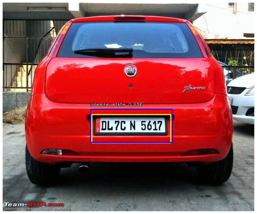
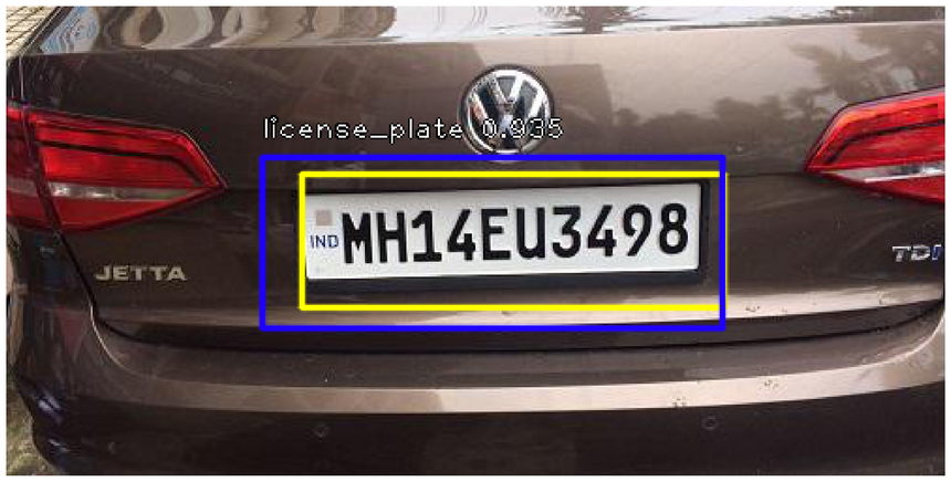
Things look pretty good. Our detected boxes are colored in blue, while the annotations are in yellow. Before jumping to conclusions, let’s have a look at another example:

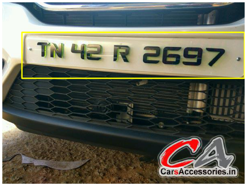
Our model didn’t detect the plate on this vehicle. Maybe it wasn’t confident enough? You can try to run the detection with a lower threshold.

Conclusion

Well done! You’ve built an Object Detector that can (somewhat) find vehicle number plates in images. You used a pre-trained model and fine tuned it on a small dataset to adapt it to the task at hand.

Here’s what you did:

• Understand Object Detection
• RetinaNet
• Prepare the Dataset
• Train a Model to Detect Vehicle Plates

Can you use the concepts you learned here and apply it to a problem/dataset you have?

Run the complete notebook in your browser

The complete project on GitHub

References

• Keras RetinaNet
• Vehicle Number Plate Detection
• Object detection: speed and accuracy comparison
• Focal Loss for Dense Object Detection
• Plate Detection —> Preparing the data
• Object Detection in Colab with Fizyr Retinanet