TL;DR Learn how to handle imbalanced data using TensorFlow 2, Keras and scikit-learn

Datasets in the wild will throw a variety of problems towards you. What are the most common ones?

The data might have too few examples, too large to fit into the RAM, multiple missing values, do not contain enough predictive power to make correct predictions, and it can imbalanced.

In this guide, we’ll try out different approaches to solving the imbalance issue for classification tasks. That isn’t the only issue on our hands. Our dataset is real, and we’ll have to deal with multiple problems - imputing missing data and handling categorical features.

Before getting any deeper, you might want to consider far simpler solutions to the imbalanced dataset problem:

• Collect more data - This might seem like a no brainer, but it is often overlooked. Can you write some more queries and extract data from your database? Do you need a few more hours for more customer data? More data can balance your dataset or might make it even more imbalanced. Either way, you want a more complete picture of the data.
• Use Tree based models - Tree-based models tend to perform better on imbalanced datasets. Essentially, they build hierarchies based on split/decision points, which might better separate the classes.

Here’s what you’ll learn:

• Impute missing data
• Handle categorical features
• Use the right metrics for classification tasks
• Set per class weights in Keras when training a model
• Use resampling techniques to balance the dataset

Run the complete code in your browser

Data

Naturally, our data should be imbalanced. Kaggle has the perfect one for us - Porto Seguro’s Safe Driver Prediction. The object is to predict whether a driver will file an insurance claim. How many drivers do that?

Setup

Let’s start with installing TensorFlow and setting up the environment:

1!pip install tensorflow-gpu
2!pip install gdown

1import numpy as np
2import tensorflow as tf
3from tensorflow import keras
4import pandas as pd
5
6RANDOM_SEED = 42
7
8np.random.seed(RANDOM_SEED)
9tf.random.set_seed(RANDOM_SEED)

We’ll use gdown to get the data from Google Drive:

1!gdown --id 18gwvNkMs6t0jL0APl9iWPrhr5GVg082S --output insurance_claim_prediction.csv

Exploration

Let’s load the data in Pandas and have a look:

1df = pd.read_csv('insurance_claim_prediction.csv')
2print(df.shape)j

1(595212, 59)

Loads of data. What features does it have?

1print(df.columns)

1Index(['id', 'target', 'ps_ind_01', 'ps_ind_02_cat', 'ps_ind_03',
2       'ps_ind_04_cat', 'ps_ind_05_cat', 'ps_ind_06_bin', 'ps_ind_07_bin',
3       'ps_ind_08_bin', 'ps_ind_09_bin', 'ps_ind_10_bin', 'ps_ind_11_bin',
4       'ps_ind_12_bin', 'ps_ind_13_bin', 'ps_ind_14', 'ps_ind_15',
5       'ps_ind_16_bin', 'ps_ind_17_bin', 'ps_ind_18_bin', 'ps_reg_01',
6       'ps_reg_02', 'ps_reg_03', 'ps_car_01_cat', 'ps_car_02_cat',
7       'ps_car_03_cat', 'ps_car_04_cat', 'ps_car_05_cat', 'ps_car_06_cat',
8       'ps_car_07_cat', 'ps_car_08_cat', 'ps_car_09_cat', 'ps_car_10_cat',
9       'ps_car_11_cat', 'ps_car_11', 'ps_car_12', 'ps_car_13', 'ps_car_14',
10       'ps_car_15', 'ps_calc_01', 'ps_calc_02', 'ps_calc_03', 'ps_calc_04',
11       'ps_calc_05', 'ps_calc_06', 'ps_calc_07', 'ps_calc_08', 'ps_calc_09',
12       'ps_calc_10', 'ps_calc_11', 'ps_calc_12', 'ps_calc_13', 'ps_calc_14',
13       'ps_calc_15_bin', 'ps_calc_16_bin', 'ps_calc_17_bin', 'ps_calc_18_bin',
14       'ps_calc_19_bin', 'ps_calc_20_bin'],
15      dtype='object')

Those seem somewhat cryptic, here is the data description:

features that belong to similar groupings are tagged as such in the feature names (e.g., ind, reg, car, calc). In addition, feature names include the postfix bin to indicate binary features and cat to indicate categorical features. Features without these designations are either continuous or ordinal. Values of -1 indicate that the feature was missing from the observation. The target columns signifies whether or not a claim was filed for that policy holder.

What is the proportion of each target class?

1no_claim, claim = df.target.value_counts()
2print(f'No claim {no_claim}')
3print(f'Claim {claim}')
4print(f'Claim proportion {round(percentage(claim, claim + no_claim), 2)}%')

1No claim 573518
2Claim 21694
3Claim proportion 3.64%

Good, we have an imbalanced dataset on our hands. Let’s look at a graphical representation of the imbalance:

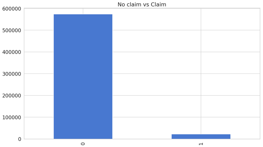
You got the visual proof right there. But how good of a model can you build using this dataset?

Baseline model

You might’ve noticed something in the data description. Missing data points have a value of -1. What should we do before training our model?

Data preprocessing

Let’s check how many rows/columns contain missing data:

1row_count = df.shape[0]
2
3for c in df.columns:
4  m_count = df[df[c] == -1][c].count()
5  if m_count > 0:
6    print(f'{c} - {m_count} ({round(percentage(m_count, row_count), 3)}%) rows missing')

1ps_ind_02_cat - 216 (0.036%) rows missing
2ps_ind_04_cat - 83 (0.014%) rows missing
3ps_ind_05_cat - 5809 (0.976%) rows missing
4ps_reg_03 - 107772 (18.106%) rows missing
5ps_car_01_cat - 107 (0.018%) rows missing
6ps_car_02_cat - 5 (0.001%) rows missing
7ps_car_03_cat - 411231 (69.09%) rows missing
8ps_car_05_cat - 266551 (44.783%) rows missing
9ps_car_07_cat - 11489 (1.93%) rows missing
10ps_car_09_cat - 569 (0.096%) rows missing
11ps_car_11 - 5 (0.001%) rows missing
12ps_car_12 - 1 (0.0%) rows missing
13ps_car_14 - 42620 (7.16%) rows missing

Missing data imputation

ps_car_03_cat, ps_car_05_cat and ps_reg_03 have too many missing rows for our own comfort. We’ll get rid of them. Note that this is not the best strategy but will do in our case.

1df.drop(
2  ["ps_car_03_cat", "ps_car_05_cat", "ps_reg_03"],
3  inplace=True,
4  axis=1
5)

What about the other features? We’ll use the SimpleImputer from scikit-learn to replace the missing values:

1from sklearn.impute import SimpleImputer
2
3cat_columns = [
4  'ps_ind_02_cat', 'ps_ind_04_cat', 'ps_ind_05_cat',
5  'ps_car_01_cat', 'ps_car_02_cat', 'ps_car_07_cat',
6  'ps_car_09_cat'
7]
8num_columns = ['ps_car_11', 'ps_car_12', 'ps_car_14']
9
10mean_imp = SimpleImputer(missing_values=-1, strategy='mean')
11cat_imp = SimpleImputer(missing_values=-1, strategy='most_frequent')
12
13for c in cat_columns:
14  df[c] = cat_imp.fit_transform(df[[c]]).ravel()
15
16for c in num_columns:
17  df[c] = mean_imp.fit_transform(df[[c]]).ravel()

We use the most frequent value for categorical features. Numerical features are replaced with the mean number of the column.

Categorical features

Pandas get_dummies() uses one-hot encoding to represent categorical features. Perfect! Let’s use it:

1df = pd.get_dummies(df, columns=cat_columns)

Now that we don’t have more missing values (you can double-check that) and categorical features are encoded, we can try to predict insurance claims. What accuracy can we get?

Building the model

We’ll start by splitting the data into train and test datasets:

1from sklearn.model_selection import train_test_split
2
3labels = df.columns[2:]
4
5X = df[labels]
6y = df['target']
7
8X_train, X_test, y_train, y_test = \
9  train_test_split(X, y, test_size=0.05, random_state=RANDOM_SEED)

Our binary classification model is a Neural Network with batch normalization and dropout layers:

1def build_model(train_data, metrics=["accuracy"]):
2  model = keras.Sequential([
3    keras.layers.Dense(
4      units=36,
5      activation='relu',
6      input_shape=(train_data.shape[-1],)
7    ),
8    keras.layers.BatchNormalization(),
9    keras.layers.Dropout(0.25),
10    keras.layers.Dense(units=1, activation='sigmoid'),
11  ])
12
13  model.compile(
14    optimizer=keras.optimizers.Adam(lr=0.001),
15    loss=keras.losses.BinaryCrossentropy(),
16    metrics=metrics
17  )
18
19  return model

You should be familiar with the training procedure:

1BATCH_SIZE = 2048
2
3model = build_model(X_train)
4history = model.fit(
5    X_train,
6    y_train,
7    batch_size=BATCH_SIZE,
8    epochs=20,
9    validation_split=0.05,
10    shuffle=True,
11    verbose=0
12)

In general, you should strive for a small batch size (e.g. 32). Our case is a bit specific - we have highly imbalanced data, so we’ll give a fair chance to each batch to contain some insurance claim data points.

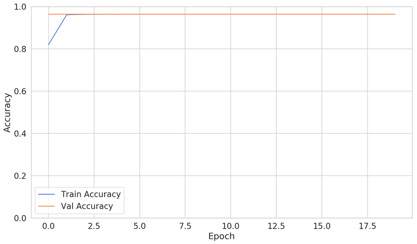
The validation accuracy seems quite good. Let’s evaluate the performance of our model:

1model.evaluate(X_test, y_test, batch_size=BATCH_SIZE)

1119043/119043 - loss: 0.1575 - accuracy: 0.9632

That’s pretty good. It seems like our model is pretty awesome. Or is it?

1def awesome_model_predict(features):
2  return np.full((features.shape[0], ), 0)
3
4y_pred = awesome_model_predict(X_test)

This amazing model predicts that there will be no claim, no matter the features. What accuracy does it get?

1from sklearn.metrics import accuracy_score
2
3accuracy_score(y_pred, y_test)

10.9632

Sweet! Wait. What? This is as good as our complex model. Is there something wrong with our approach?

Evaluating the model

Not really. We’re just using the wrong metric to evaluate our model. This is a well-known problem. The Accuracy paradox suggests accuracy might not be the correct metric when the dataset is imbalanced. What can you do?

Using the correct metrics

One way to understand the performance of our model is to use a confusion matrix. It shows us how well our model predicts for each class:

When the model is predicting everything perfectly, all values are on the main diagonal. That’s not the case. So sad! Our complex model seems as dumb as dumb as our awesome model.

Good, now we know that our model is very bad at predicting insurance claims. Can we somehow tune it to do better?

Useful metrics

We can use a wide range of other metrics to measure our peformance better:

• Precision - predicted positives divided by all positive predictions

Low precision indicates a high number of false positives.

• Recall - percentage of actual positives that were correctly classified

Low recall indicates a high number of false negatives.

• F1 score - combines precision and recall in one metric:

• ROC curve - A curve of True Positive Rate vs. False Positive Rate at different classification thresholds. It starts at (0,0) and ends at (1,1). A good model produces a curve that goes quickly from 0 to 1.

• AUC (Area under the ROC curve) - Summarizes the ROC curve with a single number. The best value is 1.0, while 0.5 is the worst.

Different combinations of precision and recall give you a better understanding of how well your model is performing for a given class:

• high precision + high recall : your model can be trusted when predicting this class
• high precision + low recall : you can trust the predictions for this class, but your model is not good at detecting it
• low precision + high recall: your model can detect the class but messes it up with other classes
• low precision + low recall : you can’t trust the predictions for this class

Measuring your model

Luckily, Keras can calculate most of those metrics for you:

1METRICS = [
2      keras.metrics.TruePositives(name='tp'),
3      keras.metrics.FalsePositives(name='fp'),
4      keras.metrics.TrueNegatives(name='tn'),
5      keras.metrics.FalseNegatives(name='fn'),
6      keras.metrics.BinaryAccuracy(name='accuracy'),
7      keras.metrics.Precision(name='precision'),
8      keras.metrics.Recall(name='recall'),
9      keras.metrics.AUC(name='auc'),
10]

And here are the results:

1loss :  0.1557253243213323
2tp :  0.0
3fp :  1.0
4tn :  57302.0
5fn :  2219.0
6accuracy :  0.9627029
7precision :  0.0
8recall :  0.0
9auc :  0.62021655
10f1 score: 0.0

Here is the ROC:

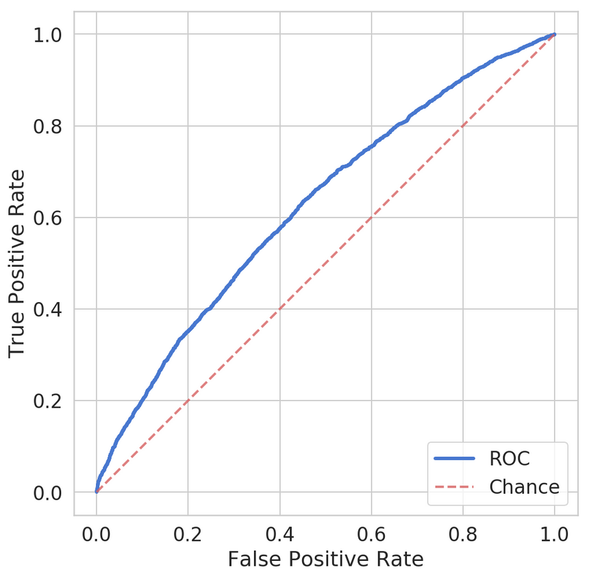
Our model is complete garbage. And we can measure how much garbage it is. Can we do better?

Weighted model

We have many more examples of no insurance claims compared to those claimed. Let’s force our model to pay attention to the underrepresented class. We can do that by passing weights for each class. First we need to calcualte those:

1no_claim_count, claim_count = np.bincount(df.target)
2total_count = len(df.target)
3
4weight_no_claim = (1 / no_claim_count) * (total_count) / 2.0
5weight_claim = (1 / claim_count) * (total_count) / 2.0
6
7class_weights = {0: weight_no_claim, 1: weight_claim}

Now, let’s use the weights when training our model:

1model = build_model(X_train, metrics=METRICS)
2
3history = model.fit(
4    X_train,
5    y_train,
6    batch_size=BATCH_SIZE,
7    epochs=20,
8    validation_split=0.05,
9    shuffle=True,
10    verbose=0,
11    class_weight=class_weights
12)

Evaluation

Let’s begin with the confusion matrix:

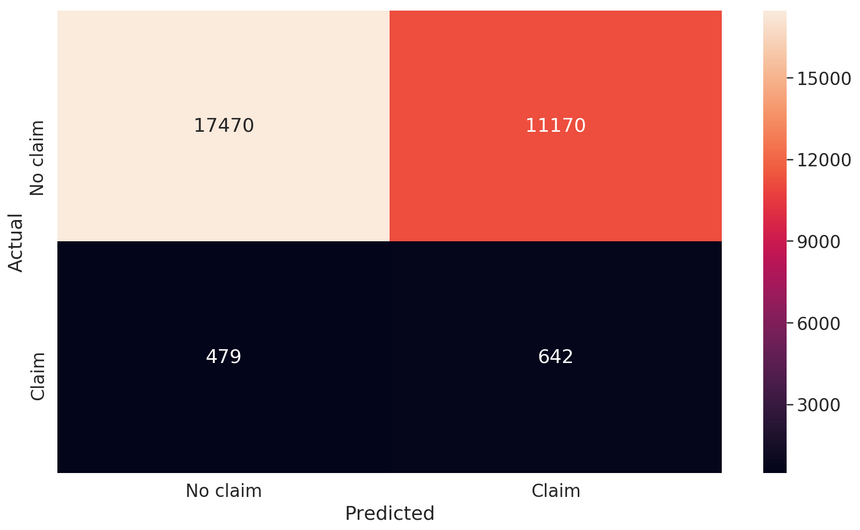
Things are a lot different now. We have a lot of correctly predicted insurance claims. The bad news is that we have a lot of predicted claims that were no claims. What can our metrics tell us?

1loss :  0.6694403463347913
2tp :  642.0
3fp :  11170.0
4tn :  17470.0
5fn :  479.0
6accuracy :  0.6085817
7precision :  0.05435151
8recall :  0.57270294
9auc :  0.63104653
10f1 score: 0.09928090930178612

The recall has jumped significantly while the precision bumped up only slightly. The F1-score is pretty low too! Overall, our model has improved somewhat. Especially, considering the minimal effort on our part. How can we do better?

Resampling techniques

These methods try to “correct” the balance in your data. They act as follows:

• oversampling - replicate examples from the under-represented class (claims)
• undersampling - sample from the most represented class (no claims) to keep only a few examples
• generate synthetic data - create new synthetic examples from the under-represented class

Naturally, a classifier trained on the “rebalanced” data will not know the original proportions. It is expected to have (much) lower accuracy since true proportions play a role in making a prediction.

You must think long and hard (that’s what she said) before using resampling methods. It can be a perfectly good approach or complete nonsense.

Let’s start by separating the classes:

1X = pd.concat([X_train, y_train], axis=1)
2
3no_claim = X[X.target == 0]
4claim = X[X.target == 1]

Oversample minority class

We’ll start by adding more copies from the “insurance claim” class. This can be a good option when the data is limited. Either way, you might want to evaluate all approaches using your metrics.

We’ll use the resample() utility from scikit-learn:

1from sklearn.utils import resample
2
3claim_upsampled = resample(claim,
4                          replace=True,
5                          n_samples=len(no_claim),
6                          random_state=RANDOM_SEED)

Here is the new distribution of no claim vs claim:

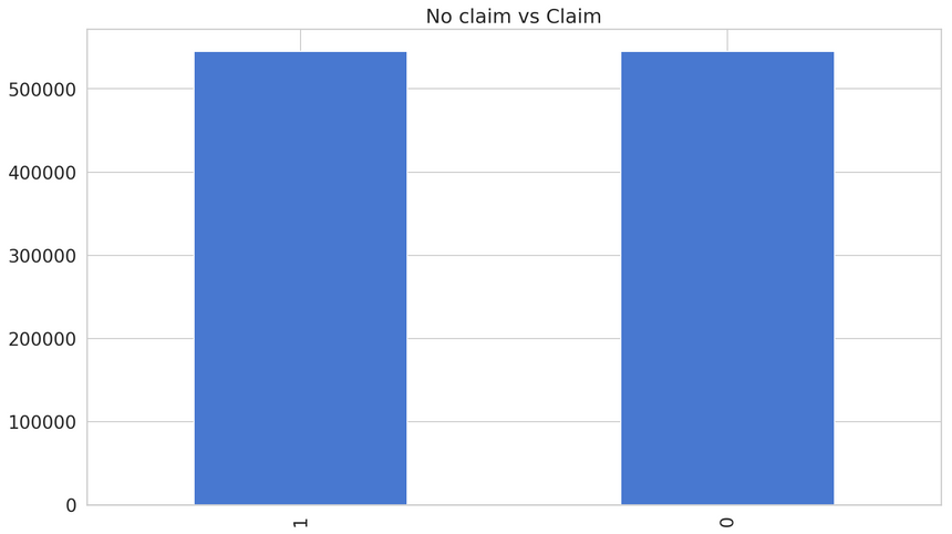
Our new model performs like this:

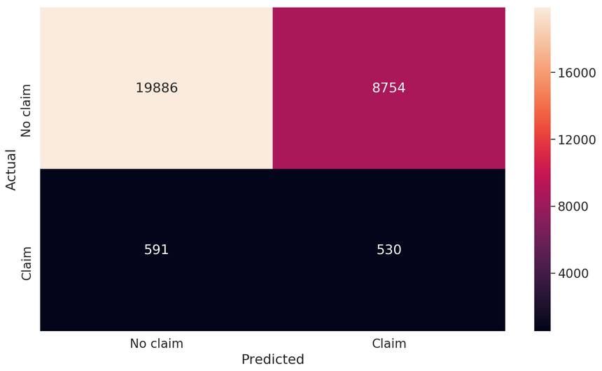
1loss :  0.6123614118771424
2tp :  530.0
3fp :  8754.0
4tn :  19886.0
5fn :  591.0
6accuracy :  0.68599844
7precision :  0.057087462
8recall :  0.47279215
9auc :  0.6274258
10f1 score: 0.10187409899086977

The performance of our model is similar to the weighted one. Can undersampling do better?

Undersample majority class

We’ll remove samples from the no claim class and balance the data this way. This can be a good option when your dataset is large. Removing data can lead to underfitting on the test set.

1no_claim_downsampled = resample(no_claim,
2                                replace = False,
3                                n_samples = len(claim),
4                                random_state = RANDOM_SEED)

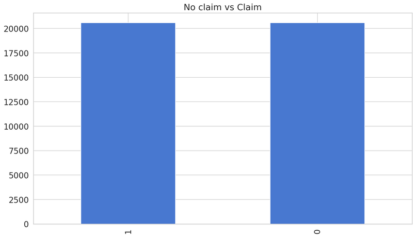
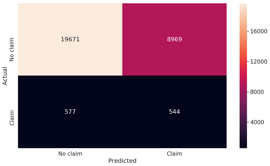
1loss :  0.6377013992475753
2tp :  544.0
3fp :  8969.0
4tn :  19671.0
5fn :  577.0
6accuracy :  0.67924464
7precision :  0.057184905
8recall :  0.485281
9auc :  0.6206339
10f1 score: 0.1023133345871732

Again, we don’t have such impressive results but doing better than the baseline model.

Generating synthetic samples

Let’s try to simulate the data generation process by creating synthetic samples. We’ll use the imbalanced-learn library to do that.

One over-sampling method to generate synthetic data is the Synthetic Minority Oversampling Technique (SMOTE). It uses KNN algorithm to generate new data samples.

1from imblearn.over_sampling import SMOTE
2
3sm = SMOTE(random_state=RANDOM_SEED, ratio=1.0)
4X_train, y_train = sm.fit_sample(X_train, y_train)

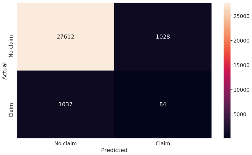
1loss :  0.26040001417683606
2tp :  84.0
3fp :  1028.0
4tn :  27612.0
5fn :  1037.0
6accuracy :  0.9306139
7precision :  0.07553957
8recall :  0.0749331
9auc :  0.5611229
10f1 score: 0.07523510971786834

We have high accuracy but very low precision and recall. Not a useful approach for our dataset.

Conclusion

There are a lot of ways to handle imbalanced datasets. You should always start with something simple (like collecting more data or using a Tree-based model) and evaluate your model with the appropriate metrics. If all else fails, come back to this guide and try the more advanced approaches.

You learned how to:

• Impute missing data
• Handle categorical features
• Use the right metrics for classification tasks
• Set per class weights in Keras when training a model
• Use resampling techniques to balance the dataset

Run the complete code in your browser

Remember that the best approach is almost always specific to the problem at hand (context is king). And sometimes, you can restate the problem as outlier/anomaly detection ;)

References

• Classification on imbalanced data

• Dealing with Imbalanced Data

• Resampling strategies for imbalanced datasets

• imbalanced-learn - Tackle the Curse of Imbalanced Datasets in Machine Learning