Curiousily

Predicting with Small Data using Bayes

05.12.2016 — R, Bayesian Statistics — 3 min read

The source of our data is “On the Use of Discriminant Functions in Taxonomy” by Alexander A. Lubischew. The dataset contains physical measures of on three species of flea beetles. The features are:

species - One of concinna, heptapotamica or heikertingeri
tars1 - width of the first joint of the first tarsus in microns
tars2 - width of the second joint of the first tarsus in microns
head - the maximal width of the head between the external edges of the eyes in 0.01 mm
aede1 - the maximal width of the aedeagus in the fore-part in microns
aede2 - the front angle of the aedeagus (1 unit = 7.5 degrees)
aede3 - the aedeagus width from the side in microns

More explanations about the dataset can be found in the Gobbi book.

This dataset is pretty small (74 rows), so we’re not in the realm of Big Data. Can we still try to make meaningful predictions about the species? Let’s find out!

Warming up

We are going to use R and JAGS to build a Bayesian model for our classification task. The model is heavily based on the excellent “Doing Bayesian Data Analysis 2nd edition” by John K. Kruschke. If you can, get this book!

Let’s import some packages into R and read our data. Please, install JAGS on your machine if you want to follow along.

1library(rjags);
2library(coda)
3library(caret)
4library(scales)
5library(ggplot2)
6library(runjags)
7library(GGally)
8library(reshape2)
9library(plyr)
10library(dplyr)
11library(parallel)
12library(mcmcplots)

1source("utils.R")
2
3seed <- 42
4set.seed(seed)
5theme_set(theme_minimal())
6options(warn=-1)

1df <- read.csv("data/flea.csv", header = T)

Exploration

Our dataset contains 74 rows with 7 variables each. We are going to answer one question: Given Flea Beetle measures what type of specie is it?

1ggplot_missing(df)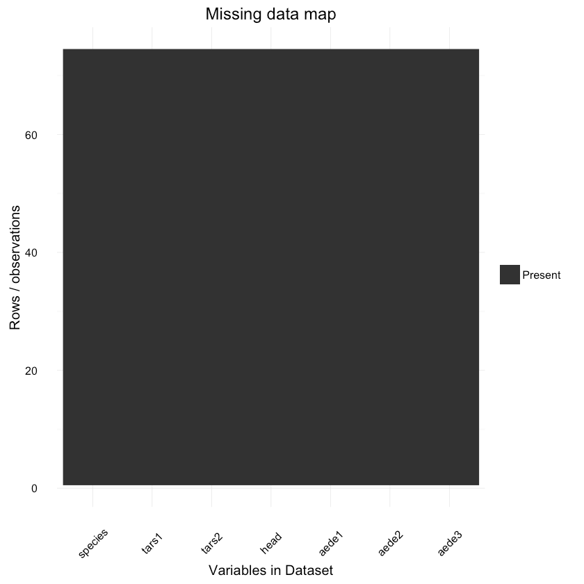

How does the features in the dataset correlate to each other?

1ggcorr(df, hjust = 0.8, layout.exp = 1) +
2    ggtitle("Correlation between Flea Beetles features")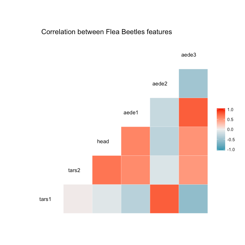

1ggplot(df, aes(x = aede2, y = species)) + geom_point() +
2    ggtitle("aede2 vs species")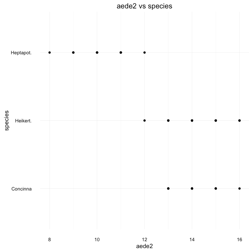

It looks like there is pretty good separation between Heptapot and the other 2 species based on aede2 alone.

1ggplot(df, aes(x = tars1, y = species)) + geom_point()  +
2    ggtitle("tars1 vs species")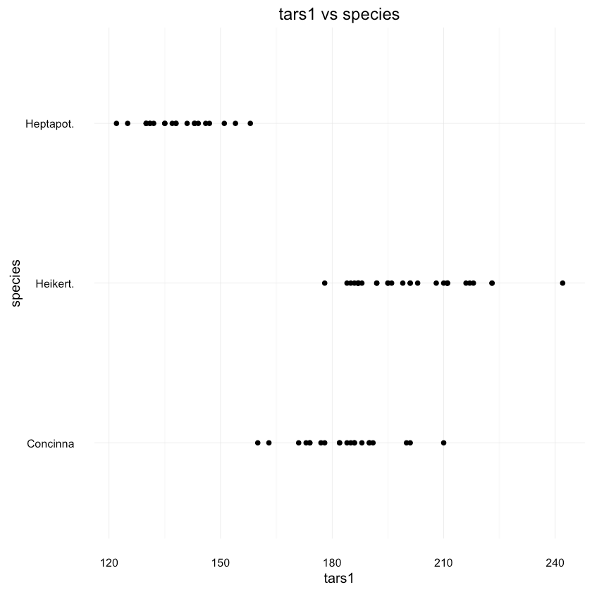

tars1 shows paints pretty similar picture. How about the species distribution in general?

1data <- as.data.frame(prop.table(table(df$species)))
2colnames(data) <- c("Species", "Percentage")
3data$Species <- unique(df$species)
4
5ggplot(data=data, aes(x=Species, y=Percentage)) +
6  geom_bar(position="dodge", stat="identity") +
7  ggtitle("Flea Beetles species distribution") +
8  scale_y_continuous(labels=percent_format())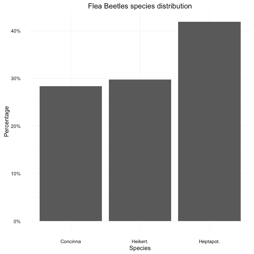

Looks ok, with lead to Heikert. Let’s not forget that our dataset is pretty small though.

Preprocessing

Now, let’s shuffle and split our data into training and testing datasets. We’ll convert the species into ints as well.

1species <- levels(df$species)
2df$species <- as.numeric(df$species)
3df <- df[sample(nrow(df)),]
4
5train_idx = createDataPartition(df$species, p=.8, list=FALSE)

1train <- df[train_idx, ]
2test <- df[-train_idx, ]
3
4y_test <- df[-train_idx, ]$species

Building our model

Now, let’s get serious and put JAGS to a test. Here is a diagram of our model:

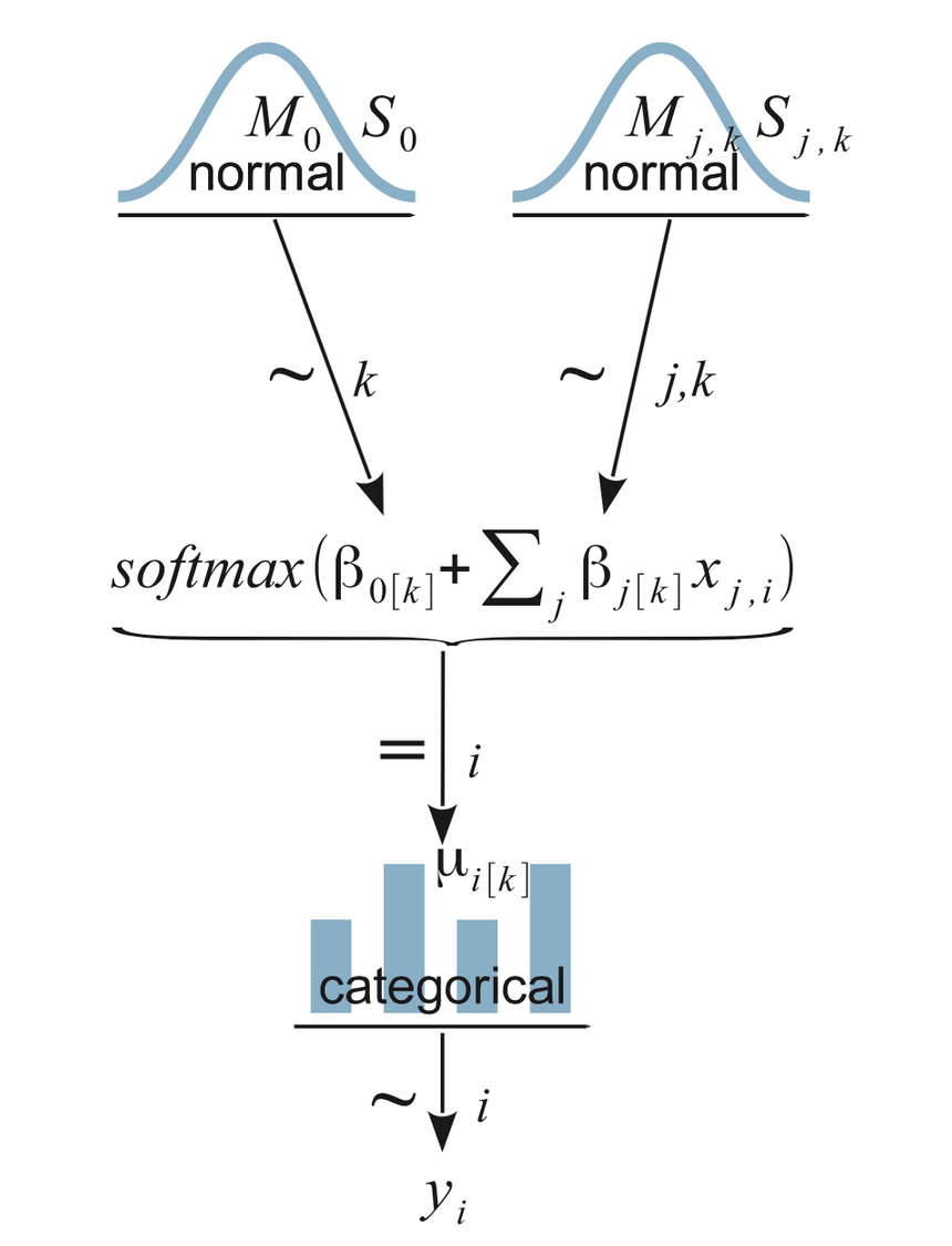
You should try to understand that bottom to top. $y_i$ is what we are trying to ultimately predict. It is a categorical distribution. Then you move to the next level (up) where the softmax is defined and finally our normally distributed vague prior distributions.

Now for our model definition. It is defined in JAGS. Almost directly taken from Kruschke’s book. So it is a string in R. First, we will standardize our input X for both training and testing data. Then, our $y_i$ is defined as categorical distribution (using dcat) that depends on our data and vague normally distributed priors.

We compute $y$ for our training and testing data within our JAGS model.

1model_string = "
2  # Standardize the data:
3  data {
4    for ( j in 1:n_features ) {
5      xm[j]  <- mean(x[,j])
6      xsd[j] <-   sd(x[,j])
7      for ( i in 1:n ) {
8        zx[i,j] <- ( x[i,j] - xm[j] ) / xsd[j]
9      }
10      # standardize the probe values:
11      for ( i in 1:n_test ) {
12        zx_test[i,j] <- (x_test[i,j] - xm[j] ) / xsd[j]
13      }
14    }
15  }
16  # Specify the model for standardized data:
17  model {
18
19    # Predicted y values at x_test:
20    for ( i in 1:n_test ) {
21      y_pred[i] ~ dcat( zy_pred[1:n_classes,i] ) # dcat normalizes its argument vector
22      for ( r in 1:n_classes ) {
23        zy_pred[r,i] <- exp( zbeta0[r] + sum( zbeta[r,1:n_features] * zx_test[i,1:n_features] ) )
24      }
25    }
26
27    for ( i in 1:n ) {
28      y[i] ~ dcat( explambda[1:n_classes,i] ) # dcat normalizes its argument vector
29      for ( r in 1:n_classes ) {
30        explambda[r,i] <- exp( zbeta0[r] + sum( zbeta[r,1:n_features] * zx[i,1:n_features] ) )
31      }
32    }
33    # Priors vague on standardized scale:
34    zbeta0[1] <- 0
35    for ( j in 1:n_features ) { zbeta[1,j] <- 0 }
36    for ( r in 2:n_classes ) { # notice starts at 2
37      zbeta0[r] ~ dnorm( 0 , 1/20^2 )
38      for ( j in 1:n_features ) {
39        zbeta[r,j] ~ dnorm( 0 , 1/20^2 )
40      }
41    }
42    # Transform to original scale:
43    for ( r in 1:n_classes ) {
44      beta[r,1:n_features] <- zbeta[r,1:n_features] / xsd[1:n_features]
45      beta0[r] <- zbeta0[r] - sum( zbeta[r,1:n_features] * xm[1:n_features] / xsd[1:n_features] )
46    }
47  }
48"

Let’s glue up everything together using runjags.

1run_mcmc = function(x, y, x_test, model,
2                    n_saved_steps=10000,
3                    thin_steps=1 ,
4                    runjags_method ,
5                    n_chains) {
6
7  # Specify the data in a list, for later shipment to JAGS:
8  data = list(
9    x = x ,
10    y = as.numeric(y) ,
11    x_test = x_test ,
12    n_test = nrow(x_test) ,
13    n_features = dim(x)[2] ,
14    n = dim(x)[1] ,
15    n_classes = length(unique(y))
16  )
17
18  writeLines(model, con="TEMPmodel.txt" )
19  #-----------------------------------------------------------------------------
20  # RUN THE CHAINS
21  parameters = c( "beta0" ,  "beta" ,
22                  "zbeta0" , "zbeta",
23                  "x_test" , "y_pred")
24
25  result <- run.jags( method=runjags_method ,
26                          model="TEMPmodel.txt" ,
27                          monitor=parameters ,
28                          data=data ,
29                          n.chains=n_chains ,
30                          adapt=500 ,
31                          burnin=1000 ,
32                          silent.jags = TRUE,
33                          sample=ceiling(n_saved_steps/n_chains) ,
34                          thin=thin_steps,
35                          summarise=FALSE ,
36                          plots=FALSE)
37  return(as.mcmc.list(result))
38}

We create a list of features (flea beetles measures) who will be used for fitting the model and the species column which we want to predict.

1n_cores = detectCores()
2if ( !is.finite(n_cores) ) { n_cores = 1 }
3if ( n_cores > 4 ) {
4  n_chains = 4  # because JAGS has only 4 rng's.
5  runjags_method = "parallel"
6}
7if ( n_cores == 4 ) {
8  n_chains = 3  # save 1 core for other processes.
9  runjags_method = "parallel"
10}
11if ( n_cores < 4 ) {
12  n_chains = 3
13  runjags_method = "rjags" # NOT parallel
14}

Properly prepare our test data and finally do some simulations

1features <- c("tars1", "tars2", "head", "aede1", "aede2", "aede3")
2
3y = train[, "species"]
4x = as.matrix(train[, features], ncol=length(x_features))
5
6x_test <- matrix(unlist(test[, features]), nrow = nrow(test), byrow = TRUE)
7
8samples = run_mcmc(x, y, x_test, model=model_string,
9                    n_saved_steps=10000,
10                    thin_steps=5,
11                    runjags_method=runjags_method,
12                    n_chains=n_chains)

1Calling 4 simulations using the parallel method...
2All chains have finished
3Simulation complete.  Reading coda files...
4Coda files loaded successfully
5Finished running the simulation

Some results

First, let’s see if our model has found a fit? Here are the traceplots for the beta parametres (our priors) in our model.

1traplot(samples, "beta");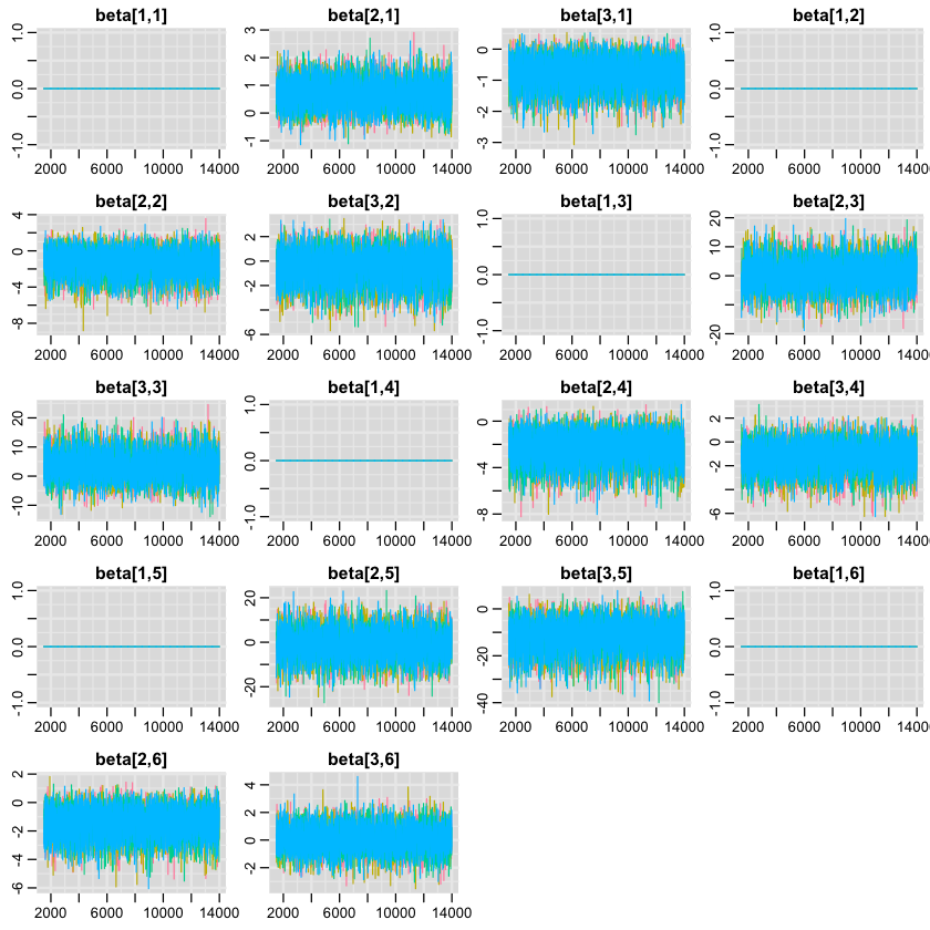

1denplot(samples, "y_pred");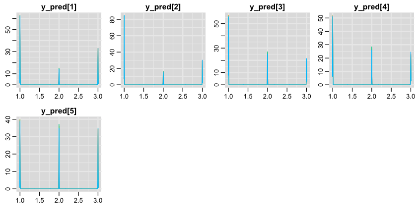

Evaluation

So, is our model good? Short answer is - no. First, let’s find all simulation results (columns in the result matrix) for our test data.

1samples_mat = as.matrix(samples)
2yp_cols = grep("y_pred", colnames(samples_mat) , value=FALSE )

And pick the most frequent value (MLE) in each column for our prediction.

1max_cols <- c()
2for(i in yp_cols) {
3  max_cols <- c(max_cols, which.max(table(samples_mat[, i]))[[1]])
4}
5
6accuracy <- data.frame(predicted = max_cols, actual=as.numeric(y_test))

1table(accuracy)

1actual
2predicted 1 2 3
3        1 2 4 2
4        2 0 4 2

1table(accuracy$predicted == accuracy$actual)

1FALSE  TRUE
2    8     6

Our accuracy is:

1table(accuracy$predicted == accuracy$actual)[[2]] / nrow(accuracy)

0.428571428571429

That sounds pretty bad. Can you improve that with another model?

Let’s have a look at a specific prediction. The main advantage of our Bayesian model is that it gives us a posterior distribution for each prediction. Think of it as a representation of uncertainty of the model’s prediction.

1data <- as.data.frame(prop.table(table(samples_mat[, ncol(samples_mat) - 1])))
2colnames(data) <- c("Species", "Percentage")
3data$Species <- species
4
5ggplot(data=data, aes(x=Species, y=Percentage)) +
6  geom_bar(position="dodge", stat="identity") +
7  ggtitle(paste("True label: ", species[y_test[length(y_test) - 1]])) +
8  scale_y_continuous(labels=percent_format())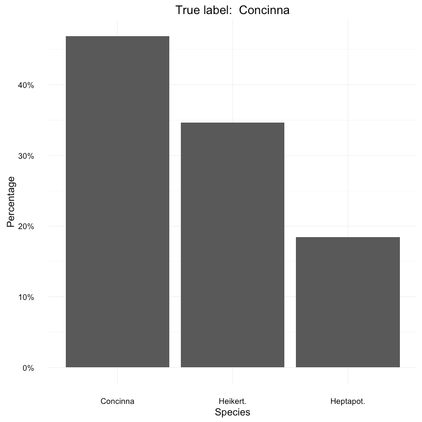

Conclusion

You made it! Well, kind of… Most probably you learned a lot, though.

Considering the size of our dataset (and that of our test data) it’s pretty unclear how well we actually did. However, that uncertainty is directly baked into the model. You can predict and roughly know how wrong you might be no matter how small/big your data size is. That is truly powerful.

References

Doing Bayesian Data Analysis
Diagnosing MCMC simulations
POLS 506: Bayesian Statistics - great course on Bayesian Stats
Frequentist example in R of Multinomial Logistic Regression
Bayesian Multiple Linear Regression Prediction in R

Want to be a Machine Learning expert?

Join the weekly newsletter on Data Science, Deep Learning and Machine Learning in your inbox, curated by me! Chosen by 10,000+ Machine Learning practitioners. (There might be some exclusive content, too!)

You'll never get spam from me

Hacker's Guide to Neural Networks in JavaScript

Build Machine Learning models (especially Deep Neural Networks) that you can easily integrate with existing or new web apps. Think of your ReactJs, Vue, or Angular app enhanced with the power of Machine Learning models.

Get SH*T Done with PyTorch

Learn how to solve real-world problems with Deep Learning models (NLP, Computer Vision, and Time Series). Go from prototyping to deployment with PyTorch and Python!

Hacker's Guide to Machine Learning with Python

This book brings the fundamentals of Machine Learning to you, using tools and techniques used to solve real-world problems in Computer Vision, Natural Language Processing, and Time Series analysis. The skills taught in this book will lay the foundation for you to advance your journey to Machine Learning Mastery!

Hands-On Machine Learning from Scratch

This book will guide you on your journey to deeper Machine Learning understanding by developing algorithms in Python from scratch! Learn why and when Machine learning is the right tool for the job and how to improve low performing models!