TL;DR Build a Logistic Regression model using Python from scratch. In the process, you will learn about the Gradient descent algorithm and use it to train your model.

Let’s say you’re developing your online clothing store. Some of your customers are already paying full price. Some don’t. You want to create a promotional campaign and offer discount codes to some customers in the hopes that this might increase your sales. But you don’t want to send discounts to customers which are likely to pay full price. How should you pick the customers that will receive discounts?

Complete source code notebook on Google Colaboratory

The Data

You collected some data from your database(s), analytics packages, etc. Here’s what you might’ve come up with:

1data = OrderedDict(
2  amount_spent =  [50,  10, 20, 5,  95,  70,  100,  200, 0],
3  send_discount = [0,   1,  1,  1,  0,   0,   0,    0,   1]
4)

Let’s load the data into a Pandas data frame:

1df = pd.DataFrame.from_dict(data)

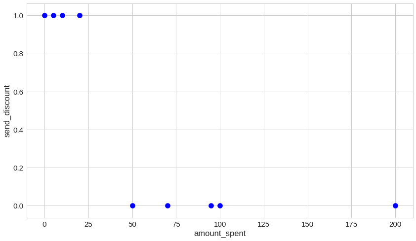
Note — the presented data is a simplification of a real dataset you might have. If your data is really simple, you might try simpler methods.

Making decisions with Logistic regression

Logistic regression is used for classification problems when the dependant/target variable is binary. That is, its values are true or false. Logistic regression is one of the most popular and widely used algorithms in practice (see this).

Some problems that can be solved with Logistic regression include:

• Email -  deciding if it is spam or not
• Online transactions  -  fraudulent or not
• Tumor classification  -  malignant or benign
• Customer upgrade  -  will the customer buy the premium upgrade or not

We want to predict the outcome of a variable y, such that:

and set 0: negative class (e.g. email is not spam) or 1: positive class (e.g. email is spam).

Can‘t we just use Linear regression?

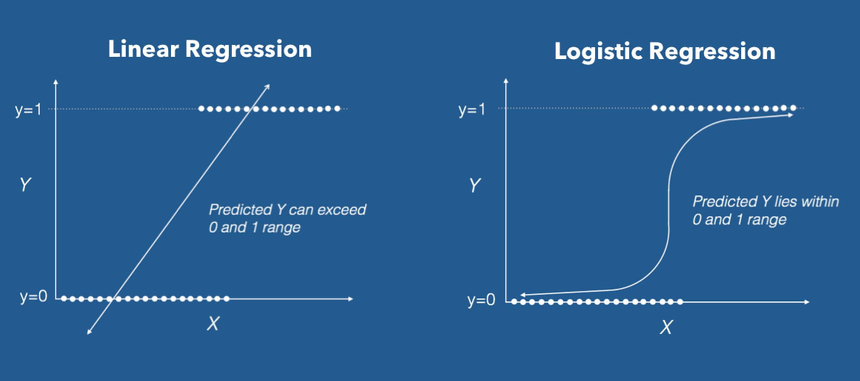source: machinelearningplus.com

Linear regression is another very popular model. It works under the assumption that the observed phenomena (your data) are explainable by a straight line.

The response variable y of the Linear regression is not restricted within the [0, 1] interval. That makes it pretty hard to take binary decisions based on its output. Thus, not suitable for our needs.

The Logistic Regression model

Given our problem, we want a model that uses 1 variable (predictor) ($x_1$ -amount_spent) to predict whether or not we should send a discount to the customer.

where the coefficients $w_i$ are paramaters of the model. Let the coeffiecient vector $W$ be:

Then we can represent $h_w(x)$ in more compact form:

That is the Linear Regression model.

We want to build a model that outputs values that are between 0 and 1, so we want to come up with a hypothesis that satisfies:

For Logistic Regression we want to modify this and introduce another function g:

We’re going to define g as:

where $z \in \mathbb{R}$. $g$ is also known as the sigmoid function or the logistic function. So, after substition, we end up with:

for our hypothesis.

A closer look at the sigmoid function

Intuitively, we’re going to use the sigmoid function “over the” Linear regression model to bound it within [0;+1].

Recall that the sigmoid function is defined as:

where $z \in \mathbb{R}$. Let’s translate that to a Python function:

1def sigmoid(z):
2  return 1 / (1 + np.exp(-z))

A graphical representation of the sigmoid function:

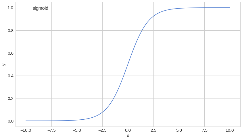
It looks familiar, right? Notice how fast it converges to -1 or +1.

How can we find the parameters for our model?

Let’s examine some approaches to find good parameters for our model. But what does good mean in this context?

Loss function

We have a model that we can use to make decisions, but we still have to find the parameters W. To do that, we need an objective measurement of how good a given set of parameters are. For that purpose, we will use a loss (cost) function:

Which is also known as the Log loss or Cross-entropy loss function

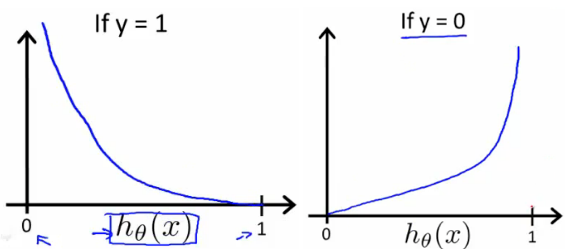source: ml-cheatsheet.readthedocs.io

We can compress the above function into one:

where

Let’s implement it in Python:

1def loss(h, y):
2  return (-y * np.log(h) - (1 - y) * np.log(1 - h)).mean()

Approach #1 — tryout a number

Let’s think of 3 numbers that represent the coefficients $w_0, w_1, w_2$.

1X = df['amount_spent'].astype('float').values
2y = df['send_discount'].astype('float').values
3
4def predict(x, w):
5  return sigmoid(x * w)
6
7def print_result(y_hat, y):
8  print(f'loss: {np.round(loss(y_hat, y), 5)} predicted: {y_hat} actual: {y}')
9
10y_hat = predict(x=X[0], w=.5)
11print_result(y_hat, y[0])

1loss: 25.0 predicted: 0.999999999986112 actual: 0.0

Unfortunately, I am pretty lazy, and this approach seems like a bit too much work for me. Let’s go to the next one:

Approach #2 — tryout a lot of numbers

Alright, these days computers are pretty fast, 6+ core laptops are everywhere. Smartphones can be pretty performant, too! Let’s use that power for good™ and try to find those pesky parameters by just trying out a lot of numbers:

1for w in np.arange(-1, 1, 0.1):
2  y_hat = predict(x=X[0], w=w)
3  print(loss(y_hat, y[0]))

10.0
20.0
30.0
46.661338147750941e-16
59.359180097590508e-14
61.3887890837434982e-11
72.0611535832696244e-09
83.059022736706331e-07
94.539889921682063e-05
100.006715348489118056
110.6931471805599397
125.006715348489103
1310.000045398900186
1415.000000305680194
1519.999999966169824
1624.99999582410784
1730.001020555434774
1834.945041100449046
19inf
20inf

Amazing, the first parameter value we tried got us a loss of 0. Is it your lucky day or this will always be the case, though? The answer is left as an exercise for the reader.

Approach #3 — Gradient descent

Gradient descent algorithms (yes, there are a lot of them) provide us with a way to find a minimum of some function f. They work by iteratively going in the direction of the descent as defined by the gradient.

In Machine Learning, we use gradient descent algorithms to find “good” parameters for our models (Logistic Regression, Linear Regression, Neural Networks, etc…).

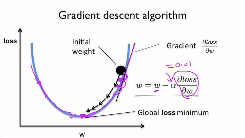source: PyTorchZeroToAll

How does it work? Starting somewhere, we take our first step downhill in the direction specified by the negative gradient. Next, we recalculate the negative gradient and take another step in the direction it specifies. This process continues until we get to a point where we can no longer move downhill  —  a local minimum.

Ok, but how can we find that gradient thing? We have to find the derivate of our cost function since our example is rather simple.

The first derivative of the sigmoid function

The first derivative of the sigmoid function is given by the following equation:

Complete derivation can be found here.

The first derivative of the cost function

Recall that the cost function was given by the following equation:

Given

We obtain the first derivative of the cost function:

Updating our parameters $W$

Now that we have the derivate, we can go back to our updating rule and use it there:

The parameter $\alpha$ is known as learning rate. High learning rate can converge quickly, but risks overshooting the lowest point. Low learning rate allows for confident moves in the direction of the negative gradient. However, it time-consuming so it will take us a lot of time to get to converge.

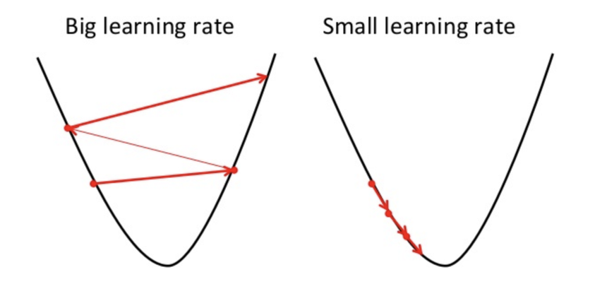source: https://towardsdatascience.com/

The Gradient descent algorithm

The algorithm we’re going to use works as follows:

1Repeat until convergence {
2  1. Calculate gradient average
3  2. Multiply by learning rate
4  3. Subtract from weights
5}

Let’s do this in Python:

1def fit(X, y, n_iter=100000, lr=0.01):
2
3  W = np.zeros(X.shape[1])
4
5  for i in range(n_iter):
6      z = np.dot(X, W)
7      h = sigmoid(z)
8      gradient = np.dot(X.T, (h - y)) / y.size
9      W -= lr * gradient
10  return W

About that until convergence part. You might notice that we kinda brute-force our way around it. That is, we will run the algorithm for a preset amount of iterations. Another interesting point is the initialization of our weights W — initially set at zero.

Let’s put our implementation to the test, literally. But first, we need a function that helps us predict y given some data X (predict whether or not we should send a discount to a customer based on its spending):

1def predict(X, W):
2  return sigmoid(np.dot(X, W))

Now for our simple test:

1class TestGradientDescent(unittest.TestCase):
2
3    def test_correct_prediction(self):
4      global X
5      global y
6      if len(X.shape) != 2:
7        X = X.reshape(X.shape[0], 1)
8      w = fit(X, y)
9      y_hat = predict(X, w).round()
10      self.assertTrue((y_hat == y).all())

Note that we use reshape to add a dummy dimension to X. Further, after our call to predict, we round the results. Recall that the sigmoid function spits out (kinda like a dragon with an upset stomach) numbers in the [0; 1] range. We’re just going to round the result in order to obtain our 0 or 1 (yes or no) answers.

1run_tests()

Here is the result of running our test case:

1F

Well, that’s not good, after all that hustling we’re nowhere near achieving our goal of finding good parameters for our model. But, what went wrong?

Welcome to your first model debugging session! Let’s start by finding whether our algorithm improves over time. We can use our loss metric for that:

1def fit(X, y, n_iter=100000, lr=0.01):
2
3  W = np.zeros(X.shape[1])
4
5  for i in range(n_iter):
6      z = np.dot(X, W)
7      h = sigmoid(z)
8      gradient = np.dot(X.T, (h - y)) / y.size
9      W -= lr * gradient
10
11      if(i % 10000 == 0):
12          e = loss(h, y)
13          print(f'loss: {e} \t')
14
15  return W

1run_tests()

We pretty much copy & pasted our training code except that we’re printing the training loss every 10,000 iterations. Let’s have a look:

1loss: 0.6931471805599453
2loss: 0.41899283818630056
3loss: 0.41899283818630056
4loss: 0.41899283818630056
5loss: 0.41899283818630056
6loss: 0.41899283818630056
7loss: 0.41899283818630056
8loss: 0.41899283818630056
9loss: 0.41899283818630056
10loss: 0.41899283818630056

1F........

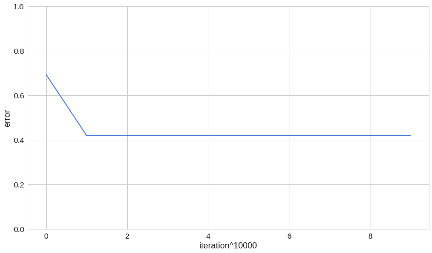
Suspiciously enough, we found a possible cause for our problem on the first try! Our loss doesn’t get low enough, in other words, our algorithm gets stuck at some point that is not a good enough minimum for us. How can we fix this? Perhaps, try out different learning rate or initializing our parameter with a different value?

First, a smaller learning rate $\alpha$ :

1def fit(X, y, n_iter=100000, lr=0.001):
2
3  W = np.zeros(X.shape[1])
4
5  for i in range(n_iter):
6      z = np.dot(X, W)
7      h = sigmoid(z)
8      gradient = np.dot(X.T, (h - y)) / y.size
9      W -= lr * gradient
10
11      if(i % 10000 == 0):
12        e = loss(h, y)
13        print(f'loss: {e} \t')
14
15  return W

1run_tests()

With $\alpha$=0.001 we obtain this:

1loss: 0.42351356323845546
2loss: 0.41899283818630056
3loss: 0.41899283818630056
4loss: 0.41899283818630056
5loss: 0.41899283818630056
6loss: 0.41899283818630056
7loss: 0.41899283818630056
8loss: 0.41899283818630056
9loss: 0.41899283818630056
10loss: 0.41899283818630056

1F.......

Not so successful, are we? How about adding one more parameter for our model to find/learn?

1def add_intercept(X):
2  intercept = np.ones((X.shape[0], 1))
3  return np.concatenate((intercept, X), axis=1)
4
5def predict(X, W):
6  X = add_intercept(X)
7  return sigmoid(np.dot(X, W))
8
9def fit(X, y, n_iter=100000, lr=0.01):
10
11  X = add_intercept(X)
12  W = np.zeros(X.shape[1])
13
14  for i in range(n_iter):
15      z = np.dot(X, W)
16      h = sigmoid(z)
17      gradient = np.dot(X.T, (h - y)) / y.size
18      W -= lr * gradient
19  return W

1run_tests()

And for the results:

1........
2
3---------------------------------------------------------
4Ran 8 tests in 0.686s
5OK

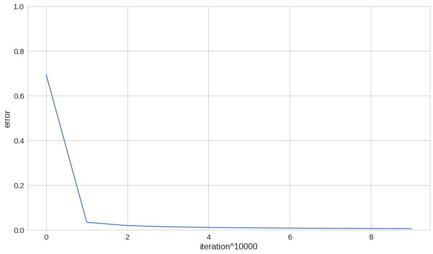
What we did here? We added a new element to our parameter vector $W$ and set it’s initial value to 1. Seems like this turn things into our favor!

Bonus — building your own LogisticRegressor

Knowing all of the details of the inner workings of the Gradient descent is good, but when solving problems in the wild, we might be hard pressed for time. In those situations, a simple & easy to use interface for fitting a Logistic Regression model might save us a lot of time. So, let’s build one!

But first, let’s write some tests:

1class TestLogisticRegressor(unittest.TestCase):
2
3    def test_correct_prediction(self):
4      global X
5      global y
6      X = X.reshape(X.shape[0], 1)
7      clf = LogisticRegressor()
8      y_hat = clf.fit(X, y).predict(X)
9      self.assertTrue((y_hat == y).all())

1class LogisticRegressor:
2
3  def _add_intercept(self, X):
4    intercept = np.ones((X.shape[0], 1))
5    return np.concatenate((intercept, X), axis=1)
6
7  def predict_probs(self, X):
8    X = self._add_intercept(X)
9    return sigmoid(np.dot(X, self.W))
10
11  def predict(self, X):
12    return self.predict_probs(X).round()
13
14  def fit(self, X, y, n_iter=100000, lr=0.01):
15
16    X = self._add_intercept(X)
17    self.W = np.zeros(X.shape[1])
18
19    for i in range(n_iter):
20        z = np.dot(X, self.W)
21        h = sigmoid(z)
22        gradient = np.dot(X.T, (h - y)) / y.size
23        self.W -= lr * gradient
24    return self

1run_tests()

We just packed all previously written functions into a tiny class. One huge advantage of this approach is the fact that we hide the complexity of the Gradient descent algorithm and the use of the parameters $W$.

Using our Regressor to decide who should receive discount codes

Now that you’re done with the “hard” part let’s use the model to predict whether or not we should send discount codes.

Let’s recall our initial data:

Now let’s try our model on data obtained from 2 new customers:

1Customer 1 - $10
2Customer 2 - $250

1X_test = np.array([10, 250])
2X_test = X_test.reshape(X_test.shape[0], 1)
3y_test = LogisticRegressor().fit(X, y).predict(X_test)

1y_test

1array([1., 0.])

Recall that 1 means send code and 0 means do not send. Looks reasonable enough. Care to try out more cases?

Complete source code notebook on Google Colaboratory

Conclusion

Well done! You have a complete (albeit simple) LogisticRegressor implementation that you can play with. Go on, have some fun with it!

Coming up next, you will implement a Linear regression model from scratch!